The principle of least action, first explicitly stated by Jacobi, is similar to Hamilton's principle, but less general and more difficult to prove. This principle is applicable only to the case when the connections and the force function do not depend on time and when, therefore, there is an integral of the living force.
This integral looks like:
Hamilton's principle stated above states that the variation of the integral

is equal to zero when the actual motion passes to any other infinitely close motion that takes the system from the same initial position to the same final position in the same time interval.
The Jacobi principle, on the contrary, expresses a property, motion, that does not depend on time. Jacobi considers the integral
defining action. The principle he established states that the variation of this integral is zero when we compare the actual motion of the system with any other infinitely close motion that takes the system from the same initial position to the same final position. In this case, we do not pay attention to the time interval spent, but we observe equation (1), i.e., the equation of manpower with the same value of the constant h as in actual movement.
This necessary extremum condition leads, generally speaking, to the minimum of the integral (2), whence comes the name of the principle of least action. The minimum condition seems to be the most natural, since the value of T is essentially positive, and therefore the integral (2) must necessarily have a minimum. The existence of a minimum can be rigorously proven only if the time interval is sufficiently small. The proof of this proposition can be found in Darboux's well-known course on the theory of surfaces. However, we will not present it here and confine ourselves to deriving the condition
432. Proof of the principle of least action.
In actual computation we encounter one difficulty which is not present in the proof of Hamilton's theorem. The variable t no longer remains independent of variation; so the variations of q i and q. are related to the variation of t by a complex relationship that follows from Eq. (1). The easiest way to get around this difficulty is to change the independent variable to one whose values lie between constant time-independent limits. Let k be a new independent variable whose limits are assumed to be independent of t. When moving the system, the parameters and t will be functions of this variable
Let the primed letters q denote the derivatives of the q parameters with respect to time.
Since the links are assumed to be independent of time, the Cartesian coordinates x, y, z are functions of q that do not contain time. Therefore their derivatives will be linear homogeneous functions of q and 7 will be a homogeneous quadratic form of q whose coefficients are functions of q. We have
![]()
In order to distinguish the time derivatives of q, we denote with parentheses, (q), the derivatives of q, taken with respect to and put in accordance with this
![]()
then we will have
![]()
and the integral (2), expressed through the new independent variable A, will take the form;

The derivative can be eliminated using the living force theorem. Indeed, the integral of the living force will be
![]()
![]()
Substituting this expression into the formula for , we bring the integral (2) to the form

The integral defining the action thus took the final form (3). The integrand is the square root of the quadratic form of the quantities
Let us show that the differential equations of the extremals of the integral (3) are exactly the Lagrange equations. The extremal equations, based on the general formulas of the calculus of variations, will be:

We multiply the equations by 2 and perform partial differentiations, taking into account that does not contain then we get, if we do not write the index ,
These are the extremal equations expressed in terms of the independent variable. The task now is to return to the independent variable
Since Г is a homogeneous function of the second degree of and is a homogeneous function of the first degree, we have
On the other hand, to the factors of derivatives in the equations of extremals, one can apply the living force theorem, which leads, as we saw above, to the substitution
![]()
As a result of all substitutions, the extremal equations are reduced to the form
![]()
![]()
We have thus arrived at the Lagrange equations.
433. The case when there are no driving forces.
In the case when there are no driving forces, there is an equation for manpower and we have

The condition that the integral is a minimum is, in this case, that the corresponding value of -10 must be the smallest. Thus, when there are no driving forces, then among all the movements in which the living force retains the same given value, the actual movement is that which brings the system from its initial position to its final position in the shortest time.
If the system is reduced to a single point moving along a fixed surface, then the actual motion, among all motions along the surface, performed at the same speed, is such a motion in which the point passes from its initial position to the final position to the shortest
time interval. In other words, a point describes on the surface the shortest line between its two positions, i.e., a geodesic line.
434. Remark.
The principle of least action assumes that the system has several degrees of freedom, since if there were only one degree of freedom, then one equation would be enough to determine the motion. Since motion can in this case be completely determined by the equation of living force, the actual motion will be the only one that satisfies this equation, and therefore cannot be compared with any other motion.

In we briefly reviewed one of the most remarkable physical principles - the principle of least action, and settled on an example that would seem to contradict it. In this article, we will explore this principle in a little more detail and see what happens in this example.
This time we need a little more math. However, I will again try to present the main part of the article at an elementary level. Slightly more strict and complex points I will highlight with color, they can be skipped without prejudice to the main understanding of the article.
Border conditions
Let's start with the simplest object - a ball moving freely in space, which is not affected by any forces. Such a ball, as is known, moves uniformly and rectilinearly. For simplicity, let's assume that it moves along the axis:
To accurately describe its motion, as a rule, initial conditions are given. For example, it is specified that at the initial moment of time the ball was at the point with the coordinate and had a speed . By setting the initial conditions in this form, we uniquely determine the further movement of the ball - it will move at a constant speed, and its position at the moment of time will be equal to the initial position plus the speed multiplied by the elapsed time: . This way of setting the initial conditions is very natural and intuitively familiar. We have given all the necessary information about the motion of the ball at the initial moment of time, and then its motion is determined by Newton's laws.
However, this is not the only way to specify the movement of the ball. Another alternative way is to specify the position of the ball at two different times and . Those. set that:
1) at the moment of time the ball was at a point (with coordinate );
2) at the moment of time the ball was at a point (with coordinate ).
The expression "was at the point" does not mean that the ball was at rest at the point. At the moment of time it could fly through the point . It means that its position at the moment of time coincided with the point . The same is true for the dot.
These two conditions also uniquely determine the motion of the ball. Its movement is easy to calculate. To satisfy both conditions, the speed of the ball must obviously be . The position of the ball at the moment of time will again be equal to the initial position plus the speed multiplied by the elapsed time:
Note that in the conditions of the problem, we did not need to set the initial speed. It was uniquely determined from conditions 1) and 2).
Setting conditions in the second way looks unusual. Perhaps it is not clear why it may be necessary to set them in this form at all. However, in the principle of least action, it is the conditions in the form 1) and 2) that are used, and not in the form of specifying the initial position and initial speed.
Trajectory with least action
Now let's digress a little from the real free motion of the ball and consider the following purely mathematical problem. Let's say we have a ball that we can manually move in any way we like. In this case, we need to satisfy conditions 1) and 2). Those. in the time interval between and we have to move it from point to point . This can be done in completely different ways. Each such way we will call the trajectory of the ball and it can be described as a function of the position of the ball from time . Let's plot several such trajectories on the graph of the position of the ball versus time:
For example, we can move the ball with the same speed equal to (green trajectory). Or we can keep it at point half the time and then move it to point at double speed (blue path). You can first move it in the opposite direction, and then move it to (brown path). You can move it back and forth (red path). In general, you can move it as you like, as long as conditions 1) and 2) are met.
For each such trajectory, we can match a number. In our example, i.e. in the absence of any forces acting on the ball, this number is equal to the total accumulated kinetic energy for the entire time of its movement in the time interval between and and is called the action.
In this case, the word "accumulated" kinetic energy does not accurately convey the meaning. In reality, the kinetic energy does not accumulate anywhere, the accumulation is used only to calculate the action for the trajectory. In mathematics, there is a very good concept for such an accumulation - the integral:As an example, let's take a 1 kg ball, set some boundary conditions and calculate the action for two different trajectories. Let the point be at a distance of 1 meter from the point , and the time is 1 second apart from the time. Those. we must move the ball, which at the initial moment of time was at the point, in one second at a distance of 1 m along the axis.The action is usually denoted by the letter . The symbol means kinetic energy. This integral means that the action is equal to the accumulated kinetic energy of the ball over the time interval from to .
In the first example (green trajectory), we moved the ball evenly, i.e. with the same speed, which, obviously, should be equal to: m / s. The kinetic energy of the ball at each moment of time is: = 1/2 J. In one second, 1/2 J of kinetic energy will accumulate. Those. action for such a trajectory is: J s.
Now let's not immediately move the ball from point to point , but hold it at point for half a second, and then, for the remaining time, evenly transfer it to point . In the first half second, the ball is at rest and its kinetic energy is zero. Therefore, the contribution to the action of this part of the trajectory is also equal to zero. For the second half second, we move the ball at double speed: m/s. The kinetic energy in this case will be equal to = 2 J. The contribution of this time interval to the action will be equal to 2 J multiplied by half a second, i.e. 1 J s. Therefore, the total action for such a trajectory is equal to J s.
Similarly, any other trajectory with the boundary conditions 1) and 2) given by us corresponds to some number equal to the action for this trajectory. Among all such trajectories, there is a trajectory with the least action. It can be proved that this trajectory is a green trajectory, i.e. uniform movement of the ball. For any other trajectory, no matter how tricky it is, the action will be greater than 1/2.
In mathematics, such a comparison for each function of a certain number is called a functional. Quite often in physics and mathematics there are problems similar to ours, i.e. to find such a function for which the value of a certain functional is minimal. For example, one of the problems that had great historical significance for the development of mathematics is the problem of the bachistochrone. Those. Finding the curve along which the ball rolls the fastest. Again, each curve can be represented by the function h(x), and each function can be assigned a number, in this case, the time the ball rolls. Again, the problem is reduced to finding a function for which the value of the functional is minimal. The branch of mathematics that deals with such problems is called the calculus of variations.
Principle of least action
In the examples discussed above, we have two special trajectories obtained in two different ways.The first trajectory is obtained from the laws of physics and corresponds to the real trajectory of a free ball, which is not affected by any forces and for which boundary conditions are set in the form 1) and 2).
The second trajectory is obtained from the mathematical problem of finding a trajectory with given boundary conditions 1) and 2) for which the action is minimal.
The principle of least action states that these two paths must coincide. In other words, if it is known that the ball moved in such a way that boundary conditions 1) and 2) were satisfied, then it necessarily moved along a trajectory for which the action is minimal compared to any other trajectory with the same boundary conditions.
This could be considered a mere coincidence. You never know the problems in which uniform trajectories and straight lines appear. However, the principle of least action turns out to be a very general principle, which is also valid in other situations, for example, for the motion of a ball in a uniform gravitational field. To do this, you only need to replace the kinetic energy with the difference between the kinetic and potential energies. This difference is called the Lagrangian or the Lagrange function and the action now becomes equal to the total accumulated Lagrangian. In fact, the Lagrange function contains all the necessary information about the dynamic properties of the system.
If we launch a ball in a uniform gravitational field in such a way that it flies past a point at time and arrives at a point at time , then it, according to Newton's laws, will fly along a parabola. It is this parabola that will coincide with the trajectories for which the action will be minimal.
Thus, for a body moving in a potential field, for example, in the gravitational field of the Earth, the Lagrange function is: . The kinetic energy depends on the speed of the body, and the potential energy depends on its position, i.e. coordinates . In analytical mechanics, the entire set of coordinates that determine the position of the system is usually denoted by one letter. For a ball moving freely in the gravitational field, means the coordinates , and .To indicate the rate of change of a quantity, in physics it is very common to simply put a dot over this quantity. For example, it denotes the rate of change of the coordinate , or, in other words, the speed of the body in the direction . Using these conventions, the speed of our ball in analytical mechanics is denoted as . Those. means velocity components.
Since the Lagrange function depends on the velocity and coordinates, and can also explicitly depend on time (explicitly depends on time, which means that the value is different at different times, for the same speeds and positions of the ball), then the action in general is written as
Not always minimal
However, at the end of the previous part, we considered an example where the principle of least action clearly does not work. To do this, we again took a free ball, on which no forces act, and placed a springy wall next to it.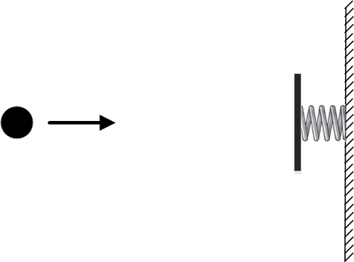
We set the boundary conditions such that the points and coincide. Those. and at the moment of time and at the moment of time the ball must be at the same point . One of the possible trajectories will be the ball standing still. Those. the entire time interval between and it will stand at the point . The kinetic and potential energy in this case will be equal to zero, so the action for such a trajectory will also be equal to zero.
Strictly speaking, potential energy can be taken equal not to zero, but to any number, since the difference in potential energy at different points in space is important. However, a change in the value of the potential energy does not affect the search for a trajectory with minimal action. It's just that for all trajectories the value of the action will change by the same number, and the trajectory with the minimum action will remain the trajectory with the minimum action. For convenience, for our ball we will choose the potential energy equal to zero.Another possible physical trajectory with the same boundary conditions would be the trajectory in which the ball first flies to the right, passing through the point at time . Then he collides with the spring, compresses it, the spring, straightening, pushes the ball back, and it again flies past the point . You can choose the speed of the ball so that, having bounced off the wall, it flew over the point exactly at the moment . The action on such a trajectory will be basically equal to the accumulated kinetic energy during the flight between the point and the wall and back. There will be some period of time when the ball compresses the spring and its potential energy increases, and during this period of time the potential energy will make a negative contribution to the action. But such a period of time will not be very large and will not greatly reduce the effect.

The figure shows both physically possible trajectories of the ball. The green trajectory corresponds to a ball at rest, while the blue one corresponds to a ball bouncing off a springy wall.
However, only one of them has a minimal effect, namely the first one! The second trajectory has more action. It turns out that in this problem there are two physically possible trajectories and only one with minimal action. Those. In this case, the principle of least action does not work.
Stationary points
To understand what's going on here, let's digress for now from the principle of least action and deal with ordinary functions. Let's take some function and draw its graph:
On the graph, I marked four special points in green. What is common for these points? Imagine that the graph of a function is a real slide along which a ball can roll. The four designated points are special in that if you place the ball exactly at this point, then it will not roll away anywhere. At all other points, for example, point E, he will not be able to stand still and will begin to slide down. Such points are called stationary. Finding such points is a useful task, since any maximum or minimum of a function, if it does not have sharp breaks, must necessarily be a stationary point.
If we classify these points more precisely, then point A is the absolute minimum of the function, i.e. its value is less than any other function value. Point B is neither a maximum nor a minimum and is called a saddle point. Point C is called a local maximum, i.e. the value in it is greater than in the neighboring points of the function. And point D is a local minimum, i.e. the value in it is less than in the neighboring points of the function.
The branch of mathematics called calculus is engaged in the search for such points. In another way, it is sometimes also called infinitesimal analysis, since it can work with infinitesimal quantities. From the point of view of mathematical analysis, stationary points have one special property, due to which they are found. To understand what this property is, we need to understand what the function looks like at very small distances from these points. To do this, we take a microscope and look into it at our points. The figure shows how the function looks in the vicinity of various points at various magnifications.

It can be seen that at very high magnification (i.e., for very small deviations of x), the stationary points look exactly the same and are very different from the non-stationary point. It is easy to understand what this difference is - the graph of a function at a stationary point becomes a strictly horizontal line with an increase, and at a non-stationary point it becomes an inclined one. That is why the ball, installed at a stationary point, will not roll.
The horizontality of a function at a stationary point can be expressed in another way: a function at a stationary point practically does not change with a very small change in its argument, even compared to the change in the argument itself. The function at a non-stationary point with a small change changes proportionally to the change. And the larger the slope of the function, the more the function changes when . In fact, as the function increases, it becomes more and more like a tangent to the graph at the point in question.
In strict mathematical language, the expression "function practically does not change at a point with a very small change" means that the ratio of the change in the function and the change in its argument tends to 0 as it tends to 0:$$display$$\lim_(∆x \to 0) \frac (∆y(x_0))(∆x) = \lim_(x \to 0) \frac (y(x_0+∆x)-y(x_0) )(∆x) = 0$$display$$
For a non-stationary point, this ratio tends to a non-zero number, which is equal to the tangent of the slope of the function at this point. The same number is called the derivative of the function at a given point. The derivative of a function shows how quickly a function changes around a given point with a small change in its argument. Thus, stationary points are points at which the derivative of a function is 0.
Stationary trajectories
By analogy with stationary points, we can introduce the concept of stationary trajectories. Recall that for each trajectory we have a certain value of the action, i.e. some number. Then there can be such a trajectory that for trajectories close to it with the same boundary conditions, the corresponding values of the action will practically not differ from the action for the most stationary trajectory. Such a trajectory is called stationary. In other words, any trajectory close to stationary will have an action value very little different from the action for that stationary trajectory.Again, in mathematical language, "slightly different" has the following precise meaning. Let us assume that we have a functional for functions with the required boundary conditions 1) and 2), i.e. and . Let us assume that the trajectory is stationary.We can take any other function such that it takes zero values at the ends, i.e. = = 0. Also take a variable , which we will make smaller and smaller. From these two functions and a variable, we can compose a third function that will also satisfy the boundary conditions and . As it decreases, the trajectory corresponding to the function will increasingly approach the trajectory .
In this case, for stationary trajectories for small, the value of the functional for the trajectories will differ very little from the value of the functional for even compared to . Those.
$$display$$\lim_(ε \to 0) \frac (S(x"(t))-S(x(t)))ε=\lim_(ε \to 0) \frac (S(x( t)+εg(t))-S(x(t)))ε = 0$$display$$
Moreover, this should be true for any trajectory satisfying the boundary conditions = = 0.The change in the functional with a small change in the function (more precisely, the linear part of the change in the functional, proportional to the change in the function) is called the variation of the functional and is denoted by . From the term "variation" comes the name "calculus of variations".
For stationary trajectories, the variation of the functional .
The method of finding stationary functions (not only for the principle of least action, but also for many other problems) was found by two mathematicians - Euler and Lagrange. It turns out that a stationary function whose functional is expressed by an integral like the action integral must satisfy a certain equation, now called the Euler-Lagrange equation.
Principle of stationary action
The situation with the minimum action for trajectories is similar to the situation with the minimum for functions. For a trajectory to have the least action, it must be a stationary trajectory. However, not all stationary trajectories are trajectories with minimal action. For example, a stationary trajectory may have a minimum action locally. Those. it will have less action than any other neighboring trajectory. However, somewhere far away there may be other trajectories for which the action will be even less.It turns out that real bodies may not necessarily move along trajectories with the least action. They can move along a wider set of special trajectories, namely, stationary trajectories. Those. the real trajectory of the body will always be stationary. Therefore, the principle of least action is more correctly called the principle of stationary action. However, according to the established tradition, it is often called the principle of least action, implying not only the minimality, but also the stationarity of trajectories.
Now we can write the principle of stationary action in mathematical language, as it is usually written in textbooks:.If we return to the example with a ball and an elastic wall, then the explanation of this situation becomes very simple now. Under the given boundary conditions that the ball must be at the point both at the time and at the time, there are two stationary trajectories. And the ball can actually move along any of these trajectories. To explicitly choose one of the trajectories, you can impose an additional condition on the motion of the ball. For example, say that the ball should bounce off the wall. Then the trajectory will be determined unambiguously.Here, are generalized coordinates, i.e. a set of variables that uniquely specify the position of the system.
- the rate of change of generalized coordinates.
- Lagrange function, which depends on the generalized coordinates, their velocities and, possibly, time.
- an action that depends on the specific trajectory of the system (i.e. from).The real trajectories of the system are stationary, i.e. for them, a variation of the action.
From the principle of least (more precisely, stationary) action, some remarkable consequences follow, which we will discuss in the next section.
When I first learned about this principle, I had a feeling of some kind of mysticism. It seems that nature mysteriously sorts through all possible ways of the system's movement and chooses the best of them.
Today I want to talk a little about one of the most remarkable physical principles - the principle of least action.
background
Since the time of Galileo, it has been known that bodies that are not acted upon by any forces move in straight lines, that is, along the shortest path. Light rays also travel in straight lines.When reflected, light also moves in such a way as to get from one point to another in the shortest way. In the picture, the shortest path will be the green path, at which the angle of incidence is equal to the angle of reflection. Any other path, such as the red one, will be longer.

This is easy to prove by simply reflecting the paths of the rays to the opposite side of the mirror. They are shown in dotted lines in the picture.

It can be seen that the green path ACB turns into a straight line ACB'. And the red path turns into a broken line ADB ', which, of course, is longer than the green one.
In 1662, Pierre Fermat suggested that the speed of light in a dense substance, such as glass, is less than in air. Prior to this, the generally accepted version was Descartes, according to which the speed of light in matter must be greater than in air in order to obtain the correct law of refraction. For Fermat, the assumption that light could move faster in a denser medium than in a rarefied one seemed unnatural. Therefore, he assumed that everything was exactly the opposite and proved an amazing thing - under this assumption, light is refracted so as to reach its destination in the minimum time.

In the figure again, the green color shows the path that the light beam actually travels. The path marked in red is the shortest, but not the fastest, because the light has a longer path to travel in the glass, and its speed is slower in it. The fastest is the actual path of the light beam.
All these facts suggested that nature acts in some rational way, light and bodies move in the most optimal way, expending as little effort as possible. But what these efforts were, and how to calculate them, remained a mystery.
In 1744, Maupertuis introduced the concept of "action" and formulated the principle according to which the true trajectory of a particle differs from any other in that the action for it is minimal. However, Maupertuis himself could not give a clear definition of what this action is equal to. A rigorous mathematical formulation of the principle of least action was developed by other mathematicians - Euler, Lagrange, and was finally given by William Hamilton:

In mathematical language, the principle of least action is formulated quite briefly, but not all readers may understand the meaning of the notation used. I want to try to explain this principle more clearly and in simpler terms.
loose body
So, imagine that you are sitting in a car at a point and at a point in time you are given a simple task: by the point in time you need to drive a car to point .
Fuel for the car is expensive and, of course, you want to spend it as little as possible. Your car is made using the latest super-technologies and can accelerate or decelerate as fast as you like. However, it is designed in such a way that the faster it goes, the more fuel it consumes. Moreover, fuel consumption is proportional to the square of speed. If you drive twice as fast, you consume 4 times more fuel in the same amount of time. In addition to speed, fuel consumption, of course, is affected by the mass of the car. The heavier our car, the more fuel it consumes. Our car's fuel consumption at each moment of time is , i.e. is exactly equal to the kinetic energy of the car.
So how do you need to drive to get to the point on time and use as little fuel as possible? It is clear that you need to go in a straight line. With an increase in the distance traveled, fuel will be consumed exactly no less. And then you can choose different tactics. For example, you can quickly arrive at the point in advance and just sit, wait for the time to come. The driving speed, and hence the fuel consumption at each moment of time, will be high, but the driving time will also be reduced. Perhaps the overall fuel consumption in this case will not be so great. Or you can go evenly, with the same speed, such that, without hurrying, exactly arrive at the moment of time. Or part of the way to go fast, and part slower. What's the best way to go?
It turns out that the most optimal, most economical way to drive is to drive at a constant speed, such as to be at the point at exactly the appointed time. Any other option will use more fuel. You can check for yourself with a few examples. The reason is that fuel consumption increases with the square of speed. Therefore, as speed increases, fuel consumption increases faster than driving time decreases, and overall fuel consumption also increases.
So, we found out that if a car consumes fuel at any given time in proportion to its kinetic energy, then the most economical way to get from point to point at exactly the appointed time is to drive evenly and in a straight line, just like a body moves in the absence of forces acting on it. forces. Any other way of driving will result in a higher overall fuel consumption.
In the field of gravity
Now let's improve our car a little. Let's attach jet engines to it so that it can fly freely in any direction. In general, the design remained the same, so the fuel consumption again remained strictly proportional to the kinetic energy of the car. If the task is now given to depart from a point at time and arrive at a point at time t, then the most economical way, as before, of course, will fly uniformly and in a straight line to arrive at the point at exactly the appointed time t. This again corresponds to the free movement of the body in three-dimensional space.
However, an unusual device was installed in the latest model of the car. This unit is able to produce fuel literally from nothing. But the design is such that the higher the car is, the more fuel the device produces at any given time. Fuel output is directly proportional to the height at which the vehicle is currently located. Also, the heavier the car, the more powerful the device is installed on it and the more fuel it produces, and the output is directly proportional to the mass of the car. The apparatus turned out to be such that the fuel output is exactly equal to (where is the free fall acceleration), i.e. potential energy of the car.
Fuel consumption at each moment of time is equal to the kinetic energy minus the potential energy of the car (minus the potential energy, because the installed vehicle produces fuel, and does not spend). Now our task is the most economical movement of the car between points and it becomes more difficult. Rectilinear uniform motion is in this case not the most effective. It turns out that it is more optimal to climb a little, linger there for a while, having developed more fuel, and then descend to the point. With the correct flight path, the total fuel consumption due to climb will cover the additional fuel costs for increasing the length of the path and increasing the speed. If calculated carefully, the most economical way for a car would be to fly in a parabola, in exactly the same trajectory and at exactly the same speed as a stone would fly in the Earth's gravity field.

Here it is worth making an explanation. Of course, it is possible to throw a stone from a point in many different ways so that it hits the point . But you need to throw it in such a way that, having flown out of a point at time , it hits a point exactly at time . It is this movement that will be the most economical for our car.
The Lagrange function and the principle of least action
Now we can transfer this analogy to real physical bodies. An analogue of the intensity of fuel consumption for bodies is called the Lagrange function or Lagrangian (in honor of Lagrange) and is denoted by the letter . The Lagrangian shows how much "fuel" the body consumes at a given time. For a body moving in a potential field, the Lagrangian is equal to its kinetic energy minus its potential energy.An analogue of the total amount of fuel consumed for the entire time of movement, i.e. the value of the Lagrangian accumulated over the entire time of motion is called the "action".
The principle of least action is that the body moves in such a way that the action (which depends on the trajectory of motion) is minimal. In this case, one should not forget that the initial and final conditions are given, i.e. where the body is at time and at time .
In this case, the body does not have to move in a uniform gravitational field, which we considered for our car. You can consider completely different situations. A body can oscillate on a rubber band, swing on a pendulum or fly around the Sun, in all these cases it moves in such a way as to minimize the "total fuel consumption" i.e. action.
If the system consists of several bodies, then the Lagrangian of such a system will be equal to the total kinetic energy of all bodies minus the total potential energy of all bodies. And again, all bodies will move in concert so that the effect of the entire system during such movement is minimal.
Not so simple
In fact, I cheated a little by saying that bodies always move in such a way as to minimize the action. Although in very many cases this is true, it is possible to think of situations in which the action is clearly not minimal.For example, let's take a ball and place it in an empty space. At some distance from it, we put an elastic wall. Let's say we want the ball to end up in the same place after some time. Under these given conditions, the ball can move in two different ways. First, he can just stay put. Secondly, you can push it towards the wall. The ball will reach the wall, bounce off it and come back. It is clear that you can push it with such speed that it will return at exactly the right time.

Both variants of the ball's motion are possible, but the action in the second case will be greater, because all this time the ball will move with non-zero kinetic energy.
How can the principle of least action be salvaged so that it holds true in such situations? We will talk about this in.
They obey him, in connection with which this principle is one of the key provisions of modern physics. The equations of motion obtained with its help are called the Euler-Lagrange equations.
The first formulation of the principle was given by P. Maupertuis in 1999, immediately pointing out its universal nature, considering it to be applicable to optics and mechanics. From this principle, he derived the laws of reflection and refraction of light.
Story
Maupertuis came to this principle from the feeling that the perfection of the universe requires a certain economy in nature and is contrary to any useless expenditure of energy. The natural motion must be such as to make some quantity a minimum. It was only necessary to find this value, which he continued to do. It was the product of the duration (time) of movement within the system by twice the amount, which we now call the kinetic energy of the system.
Euler (in "Reflexions sur quelques loix generales de la nature", 1748) adopts the principle of least action, calling action "effort". His expression in statics corresponds to what we would now call potential energy, so that his statement of least action in statics is equivalent to the minimum potential energy condition for the equilibrium configuration.
In classical mechanics
The principle of least action serves as the fundamental and standard basis for the Lagrangian and Hamiltonian formulations of mechanics.
Let's first consider the construction in such a way Lagrangian mechanics. Using the example of a physical system with one degree of freedom, we recall that an action is a functional with respect to (generalized) coordinates (in the case of one degree of freedom - one coordinate), that is, it is expressed through so that each conceivable version of the function is associated with a certain number - an action (in In this sense, we can say that an action as a functional is a rule that allows, for any given function, to calculate a well-defined number - also called an action). The action looks like:
where is the Lagrangian of the system depending on the generalized coordinate , its first derivative with respect to time , and also, possibly, explicitly on time . If the system has more degrees of freedom, then the Lagrangian depends on a larger number of generalized coordinates and their first time derivatives. Thus, the action is a scalar functional depending on the trajectory of the body.
The fact that the action is a scalar makes it easy to write it in any generalized coordinates, the main thing is that the position (configuration) of the system is uniquely characterized by them (for example, instead of Cartesian coordinates, these can be polar coordinates, distances between points of the system, angles or their functions, etc. d.).
The action can be calculated for a completely arbitrary trajectory, no matter how "wild" and "unnatural" it may be. However, in classical mechanics, among the entire set of possible trajectories, there is only one along which the body will actually go. The principle of stationarity of action just gives the answer to the question of how the body will actually move:
This means that if the Lagrangian of the system is given, then using the calculus of variations we can establish exactly how the body will move, first obtaining the equations of motion - the Euler-Lagrange equations, and then solving them. This allows not only to seriously generalize the formulation of mechanics, but also to choose the most convenient coordinates for each specific problem, not limited to Cartesian ones, which can be very useful for obtaining the simplest and most easily solved equations.
where is the Hamilton function of the given system; - (generalized) coordinates, - conjugate (generalized) impulses, characterizing together at each given moment of time the dynamic state of the system and, being each a function of time, thus characterizing the evolution (movement) of the system. In this case, to obtain the equations of motion of the system in the form of canonical Hamilton equations, it is necessary to vary the action written in this way independently for all and .
It should be noted that if it is possible in principle to find the law of motion from the conditions of the problem, then this is automatically not means that it is possible to construct a functional that takes a stationary value during true motion. An example is the joint movement of electric charges and monopoles - magnetic charges - in an electromagnetic field. Their equations of motion cannot be derived from the principle of stationarity of action. Similarly, some Hamiltonian systems have equations of motion that do not follow from this principle.
Examples
Trivial examples help evaluate the use of the operating principle through the Euler-Lagrange equations. Free particle (mass m and speed v) in Euclidean space moves in a straight line. Using the Euler-Lagrange equations, this can be shown in polar coordinates as follows. In the absence of potential, the Lagrange function is simply equal to the kinetic energy
in an orthogonal coordinate system.
In polar coordinates, the kinetic energy, and hence the Lagrange function, becomes
The radial and angular components of the equations become, respectively:
Solving these two equations
Here, is a conditional record of infinite-fold functional integration over all trajectories x(t), and is Planck's constant. We emphasize that, in principle, the action in the exponential appears (or can appear) itself, when studying the evolution operator in quantum mechanics, however, for systems that have an exact classical (non-quantum) analogue, it is exactly equal to the usual classical action.
Mathematical analysis of this expression in the classical limit - for sufficiently large , that is, for very fast oscillations of the imaginary exponent - shows that the vast majority of all possible trajectories in this integral cancel each other out in the limit (formally, at ). For almost any path, there is a path on which the phase incursion will be exactly opposite, and they will add up to zero contribution. Only those trajectories for which the action is close to the extreme value (for most systems - the minimum) are not reduced. This is a purely mathematical fact from the theory of functions of a complex variable; for example, the stationary phase method is based on it.
As a result, the particle, in full accordance with the laws of quantum mechanics, moves along all trajectories simultaneously, but under normal conditions, only trajectories that are close to stationary (that is, classical) contribute to the observed values. Since quantum mechanics becomes classical in the limit of high energies, we can assume that this is - quantum mechanical derivation of the classical principle of action stationarity.
In quantum field theory
In quantum field theory, the principle of stationarity of action is also successfully applied. The Lagrangian density here includes the operators of the corresponding quantum fields. Although it is more correct here in essence (with the exception of the classical limit and partly semiclassical) to speak not about the principle of stationarity of the action, but about Feynman integration over trajectories in the configuration or phase space of these fields - using the Lagrangian density just mentioned.
Further generalizations
More broadly, an action is understood as a functional that defines a mapping from the configuration space to the set of real numbers and, in general, it does not have to be an integral, because non-local actions are in principle possible, at least theoretically. Moreover, a configuration space is not necessarily a function space because it can have a non-commutative geometry.
2.2. Principle of least action
In the 18th century, further accumulation and systematization of scientific results took place, marked by a tendency to combine individual scientific achievements into a strictly ordered, coherent picture of the world through the systematic application of methods of mathematical analysis to the study of physical phenomena. The work of many brilliant minds in this direction has led to the creation of the basic theory of a mechanistic research program - analytical mechanics, based on the provisions of which various fundamental theories have been created that describe a specific class of con-
phenomena: hydrodynamics, elasticity theory, aerodynamics, etc. One of the most important results of analytical mechanics is the principle of least action (variational principle), which is important for understanding the processes occurring in physics at the end of the 20th century.
The roots of the emergence of variational principles in science go back to Ancient Greece and are associated with the name of Heron from Alexandria. The idea of any variational principle is to vary (change) a certain value that characterizes a given process, and select from all possible processes the one for which this value takes on an extreme (maximum or minimum) value. Heron tried to explain the laws of light reflection by varying the value characterizing the length of the path passed by a beam of light from a source to an observer when it is reflected from a mirror. He came to the conclusion that of all possible paths, a ray of light chooses the shortest (of all geometrically possible).
In the 17th century, two thousand years later, the French mathematician Fermat drew attention to Heron's principle, extended it to media with different refractive indices, and therefore reformulated it in terms of time. Fermat's principle states that in a refractive medium, the properties of which do not depend on time, a light beam passing through two points chooses a path for itself so that the time it takes to travel from the first point to the second is minimal. Heron's principle turns out to be a special case of Fermat's principle for media with a constant refractive index.
Fermat's principle attracted close attention of contemporaries. On the one hand, he was the best evidence of the "principle of economy" in nature, of the rational divine plan realized in the structure of the world, on the other hand, he contradicted Newton's corpuscular theory of light. According to Newton, it turned out that in denser media the speed of light should be greater, while it followed from Fermat's principle that in such media the speed of light becomes smaller.
In 1740, the mathematician Pierre Louis Moreau de Maupertuis, critically analyzing Fermat's principle and following the theological
logical motives about perfection and the most economical device of the Universe, proclaimed in the work “On the various laws of nature that seemed incompatible” the principle of least action. Maupertuis abandoned Fermat's shortest time and introduced a new concept - action. The action is equal to the product of the momentum of the body (momentum Р = mV) and the path traveled by the body. Time has no advantage over space, and vice versa. Therefore, light does not choose the shortest path and not the shortest time to travel it, but, according to Maupertuis, “chooses the path that gives a more real economy: the path along which it follows is the path on which the magnitude of the action is minimal.” The principle of least action was further developed in the works of Euler and Lagrange; he was the basis on which Lagrange developed a new area of mathematical analysis - the calculus of variations. This principle was further generalized and completed in the works of Hamilton. In a generalized form, the principle of least action uses the concept of action expressed not in terms of momentum, but in terms of the Lagrange function. For the case of one particle moving in some potential field, the Lagrange function can be represented as the difference of the kinetic ![]() and potential energy:
and potential energy:
(The concept of "energy" is discussed in detail in Chapter 3 of this section.)
The product is called an elementary action. The total action is the sum of all values over the entire time interval under consideration, in other words, the total action A:

The equations of motion of a particle can be obtained using the principle of least action, according to which the real motion occurs in such a way that the action turns out to be extreme, that is, its variation turns to 0:
![]()
The Lagrange-Hamilton variational principle easily allows extension to systems consisting of non-
how many (many) particles. The motion of such systems is usually considered in an abstract space (a convenient mathematical technique) of a large number of dimensions. Say, for N points, some abstract space of 3N coordinates of N particles is introduced, forming a system called the configuration space. The sequence of different states of the system is represented by a curve in this configuration space - a trajectory. Considering all possible paths connecting two given points of this 3N-dimensional space, one can make sure that the real movement of the system occurs in accordance with the principle of least action: among all possible trajectories, the one for which the action is extremal over the entire time interval of movement is realized.
When minimizing the action in classical mechanics, the Euler-Lagrange equations are obtained, the connection of which with Newton's laws is well known. The Euler-Lagrange equations for the Lagrangian of the classical electromagnetic field turn out to be Maxwell's equations. Thus, we see that the use of the Lagrangian and the principle of least action allows one to set the particle dynamics. However, the Lagrangian has one more important feature, which made the Lagrangian formalism the main one in solving almost all problems of modern physics. The fact is that along with Newtonian mechanics in physics, already in the 19th century, conservation laws were formulated for some physical quantities: the law of conservation of energy, the law of conservation of momentum, the law of conservation of angular momentum, the law of conservation of electric charge. The number of conservation laws in connection with the development of quantum physics and elementary particle physics in our century has become even greater. The question arises how to find a common basis for writing both the equations of motion (say, Newton's laws or Maxwell's equations) and the quantities conserved in time. It turned out that such a basis is the use of the Lagrangian formalism, because the Lagrangian of a particular theory turns out to be invariant (unchanged) with respect to transformations corresponding to the specific abstract space considered in this theory, which results in the conservation laws. These features of the Lagrangian
did not lead to the expediency of formulating physical theories in the language of Lagrangians. The realization of this circumstance came to physics due to the emergence of Einstein's theory of relativity.
| " |
