Expected value. mathematical expectation discrete random variable X, which takes a finite number of values Xi with probabilities Ri, is called the sum:
mathematical expectation continuous random variable X is called the integral of the product of its values X on the probability distribution density f(x):
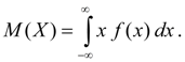 (6b)
(6b)
Improper integral (6 b) is assumed to be absolutely convergent (otherwise we say that the expectation M(X) does not exist). The mathematical expectation characterizes mean random variable X. Its dimension coincides with the dimension of a random variable.
Properties of mathematical expectation:
Dispersion. dispersion random variable X number is called:
The dispersion is scattering characteristic values of a random variable X relative to its average value M(X). The dimension of the variance is equal to the dimension of the random variable squared. Based on the definitions of variance (8) and mathematical expectation (5) for a discrete random variable and (6) for a continuous random variable, we obtain similar expressions for the variance:
 (9)
(9)
Here m = M(X).
Dispersion properties:
Standard deviation:
![]() (11)
(11)
Since the dimension of the standard deviation is the same as that of a random variable, it is more often than the variance used as a measure of dispersion.
distribution moments. The concepts of mathematical expectation and variance are special cases of a more general concept for the numerical characteristics of random variables - distribution moments. The distribution moments of a random variable are introduced as mathematical expectations of some simple functions of a random variable. So, the moment of order k relative to the point X 0 is called expectation M(X–X 0 )k. Moments relative to the origin X= 0 are called initial moments and are marked:
![]() (12)
(12)
The initial moment of the first order is the distribution center of the considered random variable:
![]() (13)
(13)
Moments relative to distribution center X= m called central moments and are marked:
![]() (14)
(14)
From (7) it follows that the central moment of the first order is always equal to zero:
The central moments do not depend on the origin of the values of the random variable, since with a shift by a constant value With its center of distribution is shifted by the same value With, and the deviation from the center does not change: X – m = (X – With) – (m – With).
Now it is obvious that dispersion- This second order central moment:
Asymmetry. Central moment of the third order:
![]() (17)
(17)
serves to evaluate distribution skewness. If the distribution is symmetrical about the point X= m, then the central moment of the third order will be equal to zero (as well as all central moments of odd orders). Therefore, if the central moment of the third order is different from zero, then the distribution cannot be symmetric. The magnitude of the asymmetry is estimated using a dimensionless asymmetry coefficient:
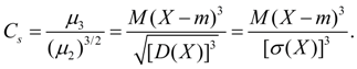 (18)
(18)
The sign of the asymmetry coefficient (18) indicates right-sided or left-sided asymmetry (Fig. 2).

Rice. 2. Types of asymmetry of distributions.
Excess. Central moment of the fourth order:
![]() (19)
(19)
serves to evaluate the so-called kurtosis, which determines the degree of steepness (pointiness) of the distribution curve near the distribution center with respect to the normal distribution curve. Since for a normal distribution, the quantity taken as kurtosis is:
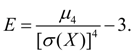 (20)
(20)
On fig. 3 shows examples of distribution curves with different values of kurtosis. For a normal distribution E= 0. Curves that are more peaked than the normal one have positive kurtosis, and those with more flat peaks have negative kurtosis.

Rice. 3. Distribution curves with different degrees of steepness (kurtosis).
Higher order moments in engineering applications of mathematical statistics are usually not used.
Fashion
discrete random variable is its most probable value. Fashion continuous a random variable is its value at which the probability density is maximum (Fig. 2). If the distribution curve has one maximum, then the distribution is called unimodal. If the distribution curve has more than one maximum, then the distribution is called polymodal. Sometimes there are distributions whose curves have not a maximum, but a minimum. Such distributions are called antimodal. In the general case, the mode and the mathematical expectation of a random variable do not coincide. In a particular case, for modal, i.e. having a mode, a symmetric distribution, and provided that there is a mathematical expectation, the latter coincides with the mode and the center of symmetry of the distribution.
Median random variable X is its meaning Me, for which equality holds: i.e. it is equally likely that the random variable X will be less or more Me. Geometrically median is the abscissa of the point at which the area under the distribution curve is divided in half (Fig. 2). In the case of a symmetric modal distribution, the median, mode, and mean are the same.
In addition to mathematical expectation and dispersion, a number of numerical characteristics are used in probability theory, reflecting certain features of the distribution.
Definition. Mode Mo(X) of a random variable X is its most probable value(for which the probability r r or probability density
If the probability or probability density reaches a maximum not at one, but at several points, the distribution is called polymodal(Fig. 3.13).

Fashion Moss), at which the probability R ( or the probability density (p(x) reaches a global maximum, is called most likely value random variable (in Fig. 3.13 this Mo(X) 2).
Definition. The median Me(X) of a continuous random variable X is its value, for which
those. the probability that the random variable X takes on a value less than the median Fur) or greater than it, the same and equal to 1/2. Geometrically vertical line X = Fur) passing through a point with an abscissa equal to Fur), divides the area of \u200b\u200bthe figure of the distribution curve into two equal parts (Fig. 3.14). Obviously, at the point X = Fur) the distribution function is equal to 1/2, i.e. P(Me(X))= 1/2 (Fig. 3.15).


Note an important property of the median of a random variable: the mathematical expectation of the absolute value of the deviation of the random variable X from the constant value C is minimal then, when this constant C is equal to the median Me(X) = m, i.e. 
(the property is similar to the property (3.10") of the minimality of the mean square of the deviation of a random variable from its mathematical expectation).
O Example 3.15. Find the mode, median and mean of a random variable X s probability density φ(x) = 3x 2 for xx.
Decision. The distribution curve is shown in fig. 3.16. Obviously, the probability density φ(x) is maximum at X= Mo(X) = 1.
median Fur) = b we find from condition (3.28):

where 
The mathematical expectation is calculated by the formula (3.25):
Mutual arrangement of points M(X) > Me(X) and Moss) in ascending order of abscissa is shown in fig. 3.16. ?
Along with the numerical characteristics noted above, the concept of quantiles and percentage points is used to describe a random variable.
Definition. Level quantile y-quantile )
is called such a value x q of a random variable , at which its distribution function takes a value equal to d, i.e.
Some quantiles have received a special name. Obviously, the above median random variable is the 0.5 level quantile, i.e. Me (X) \u003d x 05. The quantiles dg 0 2 5 and x 075 are named respectively lower and upper quartileK
Closely related to the concept of a quantile is the concept percentage point. Under YuOuHo-noi dot
implied quantile x x (( ,
those. such a value of a random variable x,
under which ![]()
0 Example 3.16. According to example 3.15 find the quantile x 03 and 30% random variable point x.
Decision. According to formula (3.23), the distribution function
We find the quantile r 0 z from equation (3.29), i.e. x$ 3 \u003d 0.3, from where L "oz -0.67. Find the 30% point of the random variable x, or quantile x 0 7, from the equation x$ 7 = 0.7, whence x 0 7 "0.89. ?
Among the numerical characteristics of a random variable, the moments - initial and central - are of particular importance.
Definition. Starting momentk-th order of a random variable X is the mathematical expectation of the k-th power of this variable :
Definition. Central momentthe k-th order of a random variable X is the mathematical expectation of the k-th degree of deviation of the random variable X from its mathematical expectation:
Formulas for calculating the moments for discrete random variables (taking the values x 1 with probabilities p,) and continuous (with probability density cp(x)) are given in Table. 3.1.
Table 3.1
It is easy to see that when k = 1 first initial moment of random variable X is its mathematical expectation, i.e. h x \u003d M [X) \u003d a, at to= 2 the second central moment is the dispersion, i.e. p 2 = T)(X).
The central moments p A can be expressed in terms of the initial moments using the formulas:
etc. 
For example, c 3 \u003d M (X-a) * \u003d M (X * -ZaX 2 + Za 2 X-a-\u003e) \u003d M (X *) ~ -ZaM (X 2) + Za 2 M (X) ~ a3 \u003d y 3 -Zy ^ + Zy (y, -y ^ \u003d y 3 - Zy ^ + 2y ^ (when deriving, we took into account that a = M(X)= V, - non-random value). ?
As noted above, the mathematical expectation M(X), or the first initial moment, characterizes the average value or position, the center of distribution of a random variable X on the number line; dispersion OH), or the second central moment p 2 , - s t s - distribution scattering X relatively M(X). Higher-order moments serve for a more detailed description of the distribution.
Third central moment p 3 serves to characterize the asymmetry of the distribution (skewness). It has the dimension of a cube of a random variable. To get a dimensionless value, it is divided by about 3, where a is the standard deviation of the random variable x. Received value BUT called coefficient of asymmetry of a random variable.
If the distribution is symmetrical with respect to the mathematical expectation, then the asymmetry coefficient is A = 0.
On fig. 3.17 shows two distribution curves: I and II. Curve I has a positive (right-sided) asymmetry (L > 0), and curve II has a negative (left-sided) (L 

Fourth central moment p 4 serves to characterize the steepness (peak of the top or flat top - post) of the distribution.
fashion() continuous random variable is its value, which corresponds to the maximum value of its probability density.
median() A continuous random variable is its value, which is determined by the equality:
B15. Binomial distribution law and its numerical characteristics. Binomial distribution describes repeated independent experiences. This law determines the occurrence of an event times in independent trials, if the probability of the occurrence of an event in each of these experiments does not change from experience to experience. Probability:
![]() ,
,
where: is the known probability of the occurrence of an event in the experiment, which does not change from experience to experience;
is the probability of the event not appearing in the experiment;
![]() is the specified number of occurrence of the event in the experiments;
is the specified number of occurrence of the event in the experiments;
![]() is the number of combinations of elements by .
is the number of combinations of elements by .
B15. Uniform distribution law, graphs of the distribution function and density, numerical characteristics. A continuous random variable is considered evenly distributed, if its probability density has the form:

Expected value random variable with uniform distribution:
Dispersion can be calculated as follows:
Standard deviation will look like:
![]() .
.
B17. The exponential law of distribution, graphs of the function and distribution density, numerical characteristics. exponential distribution A continuous random variable is a distribution that is described by the following expression for the probability density:
 ,
,
where is a constant positive value.
The probability distribution function in this case has the form:
![]()
The mathematical expectation of a random variable with an exponential distribution is obtained based on the general formula, taking into account the fact that when:
![]() .
.
Integrating this expression by parts, we find: .
The variance for the exponential distribution can be obtained using the expression:
![]() .
.
Substituting the expression for the probability density, we find:
![]()
Calculating the integral by parts, we get: .
B16. Normal distribution law, graphs of the function and distribution density. Standard normal distribution. Reflected normal distribution function. normal such a distribution of a random variable is called, the probability density of which is described by the Gaussian function:

where is the standard deviation;
is the mathematical expectation of a random variable.
 |
A normal distribution density plot is called a normal Gaussian curve.
B18. Markov's inequality. Generalized Chebyshev's inequality. If for a random variable X exists, then for any Markov's inequality ![]() .
.
It stems from generalized Chebyshev inequality: Let the function be monotonically increasing and non-negative on . If for a random variable X exists, then for any the inequality ![]() .
.
B19. The law of large numbers in the form of Chebyshev. Its meaning. Consequence of the law of large numbers in the form of Chebyshev. The law of large numbers in Bernoulli form. Under law of large numbers in probability theory, a number of theorems are understood, in each of which the fact of an asymptotic approximation of the average value of a large number of experimental data to the mathematical expectation of a random variable is established. The proofs of these theorems are based on Chebyshev's inequality. This inequality can be obtained by considering a discrete random variable with possible values .
Theorem. Let there be a finite sequence ![]() independent random variables, with the same mathematical expectation and variances limited by the same constant :
independent random variables, with the same mathematical expectation and variances limited by the same constant :
Then, whatever the number , the probability of the event
![]()
tends to unity at .
Chebyshev's theorem establishes a connection between probability theory, which considers the average characteristics of the entire set of values of a random variable, and mathematical statistics, which operates on a limited set of values of this variable. It shows that for a sufficiently large number of measurements of a certain random variable, the arithmetic mean of the values of these measurements approaches the mathematical expectation.
IN 20. Subject and tasks of mathematical statistics. General and sample populations. Selection method. Math statistics- the science of mathematical methods of systematization and use of statistical data for scientific and practical conclusions, based on the theory of probability.
The objects of study of mathematical statistics are random events, quantities and functions that characterize the considered random phenomenon. The following events are random: winning one ticket of the cash lottery, compliance of the controlled product with the established requirements, trouble-free operation of the car during the first month of its operation, fulfillment by the contractor of the daily work schedule.
sampling set is a collection of randomly selected objects.
General population name the set of objects from which the sample is made.
AT 21. Selection methods.
Methods of selection: 1 Selection that does not require the division of the general population into parts. These include a) simple random non-repetitive selection and b) simple random reselection. 2) Selection, in which the general population is divided into parts. These include a) type selection, b) mechanical selection and c) serial selection.
Simple random called selection, in which objects are extracted one by one from the general population.
Typical called selection, in which objects are selected not from the entire general population, but from each of its “typical” parts.
Mechanical called selection, in which the general population is mechanically divided into as many groups as there are objects to be included in the sample, and one object is selected from each group.
Serial called selection, in which objects are selected from the general population not one at a time, but "series", which are subjected to a continuous survey.
B22. Statistical and variational series. Empirical distribution function and its properties. Variational series for discrete and continuous random variables. Let a sample be taken from the general population, and the value of the parameter under study was observed once, - once, etc. However, the sample size The observed values are called options, and the sequence is a variant written in ascending order - variational series. The number of observations is called frequencies, and their relationship to the sample size - relative frequencies.Variation series can be represented as a table:
| X | ….. | |||
| n | …. |
The statistical distribution of the sample call the list of options and their respective relative frequencies. The statistical distribution can be represented as:
| X | ….. | |||
| w | …. |
where are the relative frequencies .
Empirical distribution function call the function that determines for each value x the relative frequency of the event X The purpose of the lesson: to form students' understanding of the median of a set of numbers and the ability to calculate it for simple numerical sets, fixing the concept of the arithmetic mean set of numbers. Lesson type: explanation of new material. Equipment: board, textbook, ed. Yu.N Tyurina “Probability theory and statistics”, computer with projector. Inform the topic of the lesson and formulate its objectives. Questions for students: Oral tasks: Find the arithmetic mean of a set of numbers: Checking homework with a projector ( Appendix 1): Textbook:: No. 12 (b, d), No. 18 (c, d) In the previous lesson, we got acquainted with such a statistical characteristic as the arithmetic mean of a set of numbers. Today we will devote a lesson to another statistical characteristic - the median. Not only the arithmetic mean shows where on the number line the numbers of any set are located and where their center is. Another indicator is the median. The median of a set of numbers is the number that divides the set into two equal parts. Instead of "median" one could say "middle". First, using examples, we will analyze how to find the median, and then we will give a strict definition. Consider the following oral example using a projector ( Annex 2)
At the end of the school year, 11 students of the 7th grade passed the standard for running 100 meters. The following results were recorded: After the guys ran the distance, Petya approached the teacher and asked what his result was. “Most average: 16.9 seconds,” the teacher replied "Why?" Petya was surprised. - After all, the arithmetic mean of all the results is about 18.3 seconds, and I ran a second or more better. And in general, Katya’s result (18.4) is much closer to the average than mine.” “Your result is average because five people ran better than you and five worse. So you are right in the middle,” the teacher said. [ 2 ] Write an algorithm for finding the median of a set of numbers: Invite students to independently formulate the definition of the median of a set of numbers, then read two definitions of the median in the textbook (p. 50), then analyze examples 4 and 5 of the textbook (pp. 50-52) Comment: Draw students' attention to an important circumstance: the median is practically insensitive to significant deviations of individual extreme values of sets of numbers. In statistics, this property is called stability. The stability of a statistical indicator is a very important property, it insures us against random errors and individual unreliable data. The decision of numbers from the textbook to item 11 "Median". Set of numbers: 1,3,5,7,9 =(1+3+5+7+9):5=25:5=5 Set of numbers: 1,3,5,7,14. =(1+3+5+7+14):5=30:5=6 a) Set of numbers: 3,4,11,17,21 b) Set of numbers: 17,18,19,25,28 c) Set of numbers: 25, 25, 27, 28, 29, 40, 50 Conclusion: the median of a set of numbers consisting of an odd number of members is equal to the number in the middle. a) Set of numbers: 2, 4, 8
, 9. Me = (4+8):2=12:2=6 b) Set of numbers: 1,3, 5,7
,8,9. Me = (5+7):2=12:2=6 The median of a set of numbers containing an even number of members is half the sum of the two numbers in the middle. The student received the following grades in algebra during the quarter: 5, 4, 2, 5, 5, 4, 4, 5, 5, 5. Find the mean score and median of this set. [ 3 ] Let's order a set of numbers: 2,4,4,4,5,5,5,5,5,5 Only 10 numbers, to find the median you need to take two middle numbers and find their half sum. Me = (5+5):2 = 5 Question to students: If you were a teacher, what grade would you give this student for a quarter? Justify the answer. The president of the company receives a salary of 300,000 rubles. three of his deputies receive 150,000 rubles each, forty employees - 50,000 rubles each. and the salary of a cleaner is 10,000 rubles. Find the arithmetic mean and median of salaries in the company. Which of these characteristics is more profitable for the president to use for advertising purposes? = (300000+3 150000+40 50000+10000):(1+3+40+1) = 2760000:4561333.33 (rubles) Task 3. (Invite students to solve on their own, project the task using a projector) The table shows the approximate volume of water in the largest lakes and reservoirs in Russia in cubic meters. km. (Appendix 3)
[ 4 ] A) Find the average volume of water in these reservoirs (arithmetic mean); B) Find the volume of water in the average size of the reservoir (median of the data); C) In your opinion, which of these characteristics - the arithmetic mean or the median - best describes the volume of a typical large Russian reservoir? Explain the answer. a) 2459 cu. km b) 60 cu. km c) Median, because data contains values that are very different from all others. Task 4. Orally. A) How many numbers are in the set if its median is its ninth term? B) How many numbers are in the set if its median is the arithmetic mean of the 7th and 8th members? C) In a set of seven numbers, the largest number was increased by 14. Will this change both the arithmetic mean and the median? D) Each of the numbers in the set has been increased by 3. What will happen to the arithmetic mean and median? Sweets in the store are sold by weight. To find out how many sweets are contained in one kilogram, Masha decided to find the weight of one candy. She weighed several candies and got the following results: 12, 13, 14, 12, 15, 16, 14, 13, 11. Both characteristics are suitable for estimating the weight of one candy, since they are not very different from each other. So, to characterize statistical information, the arithmetic mean and median are used. In many cases, some of the characteristics may not have any meaningful meaning (for example, having information about the time of road accidents, it hardly makes sense to talk about the arithmetic mean of these data). Literature: Fashion- the value in the set of observations that occurs most often Mo \u003d X Mo + h Mo * (f Mo - f Mo-1) : ((f Mo - f Mo-1) + (f Mo - f Mo + 1)), here X Mo is the left border of the modal interval, h Mo is the length of the modal interval, f Mo-1 is the frequency of the premodal interval, f Mo is the frequency of the modal interval, f Mo+1 is the frequency of the postmodal interval. The mode of an absolutely continuous distribution is any point of the local maximum of the distribution density. For discrete distributions, a mode is any value a i whose probability p i is greater than the probabilities of neighboring values Median continuous random variable X its value Me is called such, for which it is equally probable whether the random variable will turn out to be less or more Me, i.e. M e \u003d (n + 1) / 2 P(X < Me) = P(X > Me) Evenly distributed NEW Even distribution. A continuous random variable is called uniformly distributed on the segment () if its distribution density function (Fig. 1.6, a) looks like: Designation: - SW is distributed uniformly on . Accordingly, the distribution function on the segment (Fig. 1.6, b): Rice. 1.6. Functions of a random variable distributed uniformly on [ a,b]: a– probability densities f(x); b– distributions F(x) The mathematical expectation and variance of this RV are determined by the expressions: Due to the symmetry of the density function, it coincides with the median. Fashion has no uniform distribution Example 4
The waiting time for an answer to a phone call is a random variable that obeys a uniform distribution law in the range from 0 to 2 minutes. Find the integral and differential distribution functions of this random variable. 27. Normal law of probability distribution A continuous random variable x has a normal distribution with parameters: m,s > 0, if the probability distribution density has the form: where: m is the mathematical expectation, s is the standard deviation. The normal distribution is also called Gaussian after the German mathematician Gauss. The fact that a random variable has a normal distribution with parameters: m, , is denoted as follows: N (m, s), where: m=a=M[X]; Quite often, in formulas, the mathematical expectation is denoted by a
. If a random variable is distributed according to the law N(0,1), then it is called a normalized or standardized normal value. The distribution function for it has the form: The graph of the density of the normal distribution, which is called the normal curve or Gaussian curve, is shown in Fig. 5.4. Rice. 5.4. Normal distribution density properties a random variable with a normal distribution law. 1. If , then to find the probability that this value falls into a given interval ( x 1; x 2) the formula is used: 2. The probability that the deviation of a random variable from its mathematical expectation will not exceed the value (in absolute value) is equal to.During the classes
1. Organizational moment.
2. Actualization of previous knowledge.
3. Learning new material.
4. Consolidation of the studied material.
![]()
