Iteration method. In this method, a comparison is made with a certain database, where for each of the objects there are different options for modifying the display. For example, for optical image recognition, you can apply the iteration method at different angles or scales, offsets, deformations, etc. For letters, you can iterate over the font or its properties. In the case of sound pattern recognition, there is a comparison with some known patterns (a word spoken by many people). Further, a deeper analysis of the characteristics of the image is performed. In the case of optical recognition, this may be the definition of geometric characteristics. The sound sample in this case is subjected to frequency and amplitude analysis.

The next method is use of artificial neural networks(INS). It requires either a huge number of examples of the recognition task, or a special neural network structure that takes into account the specifics of this task. But, nevertheless, this method is characterized by high efficiency and productivity.

Methods based on estimates of the distribution densities of feature values. Borrowed from the classical theory of statistical decisions, in which the objects of study are considered as realizations of a multidimensional random variable distributed in the feature space according to some law. They are based on the Bayesian decision-making scheme, which appeals to the initial probabilities of objects belonging to a particular class and conditional feature distribution densities.

The group of methods based on the estimation of the distribution densities of feature values ​​is directly related to the methods of discriminant analysis. The Bayesian approach to decision making is one of the most developed parametric methods in modern statistics, for which the analytical expression of the distribution law (the normal law) is considered to be known and only a small number of parameters (mean vectors and covariance matrices) need to be estimated. The main difficulties in applying this method are considered to be the need to remember the entire training set to calculate density estimates and high sensitivity to the training set.

Methods based on assumptions about the class of decision functions. In this group, the type of the decision function is considered to be known and its quality functional is given. Based on this functional, the optimal approximation to the decision function is found from the training sequence. The decision rule quality functional is usually associated with an error. The main advantage of the method is the clarity of the mathematical formulation of the recognition problem. The possibility of extracting new knowledge about the nature of an object, in particular, knowledge about the mechanisms of interaction of attributes, is fundamentally limited here by a given structure of interaction, fixed in the chosen form of decision functions.

Prototype comparison method. This is the easiest extensional recognition method in practice. It applies when the recognizable classes are shown as compact geometric classes. Then the center of the geometric grouping (or the object closest to the center) is chosen as the prototype point.

To classify an indefinite object, the nearest prototype is found, and the object belongs to the same class as it. Obviously, no generalized images are formed in this method. Various types of distances can be used as a measure.

Method of k nearest neighbors. The method lies in the fact that when classifying an unknown object, a given number (k) of geometrically nearest feature space of other nearest neighbors with already known belonging to a class is found. The decision to assign an unknown object is made by analyzing information about its nearest neighbors. The need to reduce the number of objects in the training sample (diagnostic precedents) is a disadvantage of this method, since this reduces the representativeness of the training sample.

Based on the fact that different recognition algorithms behave differently on the same sample, the question arises of a synthetic decision rule that would use the strengths of all algorithms. For this, there is a synthetic method or sets of decision rules that combine the most positive aspects of each of the methods.

In conclusion of the review of recognition methods, we present the essence of the above in a summary table, adding some other methods used in practice.

Table 1. Classification table of recognition methods, comparison of their areas of application and limitations

Classification of recognition methods	Application area	Limitations (disadvantages)
Intensive recognition methods	Methods based on density estimates	Problems with a known distribution (normal), the need to collect large statistics	The need to enumerate the entire training set during recognition, high sensitivity to non-representativeness of the training set and artifacts
Assumption based methods	Classes should be well separable	The form of the decision function must be known in advance. The impossibility of taking into account new knowledge about correlations between features
Boolean Methods	Problems of small dimension	When selecting logical decision rules, a complete enumeration is necessary. High labor intensity
Linguistic Methods		The task of determining the grammar for a certain set of statements (descriptions of objects) is difficult to formalize. Unresolved theoretical problems
Extensional methods of recognition	Prototype comparison method	Problems of small dimension of feature space	High dependence of classification results on the metric. Unknown optimal metric
k nearest neighbor method		High dependence of classification results on the metric. The need for a complete enumeration of the training sample during recognition. Computational complexity
Grade Calculation Algorithms (ABO)	Problems of small dimension in terms of the number of classes and features	Dependence of classification results on the metric. The need for a complete enumeration of the training sample during recognition. High technical complexity of the method
Collective decision rules (CRC) is a synthetic method.	Problems of small dimension in terms of the number of classes and features	Very high technical complexity of the method, the unresolved number of theoretical problems, both in determining the areas of competence of particular methods, and in the particular methods themselves

Lecture number 17.PATTERN RECOGNITION METHODS

There are the following groups of recognition methods:

Proximity Function Methods

Discriminant Function Methods

Statistical methods of recognition.

Linguistic Methods

heuristic methods.

The first three groups of methods are focused on the analysis of features expressed as numbers or vectors with numerical components.

The group of linguistic methods provides pattern recognition based on the analysis of their structure, which is described by the corresponding structural features and relationships between them.

The group of heuristic methods combines the characteristic techniques and logical procedures used by humans in pattern recognition.

Proximity Function Methods

The methods of this group are based on the use of functions that evaluate the measure of proximity between the recognizable image and the vector x * = (x * 1 ,….,x*n), and reference images of various classes, represented by vectors x i = (x i 1 ,…, x i n), i= 1,…,N, where i- image class number.

The recognition procedure according to this method consists in calculating the distance between the point of the recognized image and each of the points representing the reference image, i.e. in the calculation of all values d i , i= 1,…,N. The image belongs to the class for which the value d i has the least value among all i= 1,…,N .

A function that maps each pair of vectors x i, x * a real number as a measure of their closeness, i.e. determining the distance between them can be quite arbitrary. In mathematics, such a function is called the space metric. It must satisfy the following axioms:

r(x,y)=r(y,x);

r(x,y) > 0 if x not equal y and r(x,y)=0 if x=y;

r(x,y) <=r(x,z)+r(z,y)

These axioms are satisfied, in particular, by the following functions

a i= 1/2 , j=1,2,…n.

b i=sum, j=1,2,…n.

c i=max abs( x i‑ x j *), j=1,2,…n.

The first of these is called the Euclidean norm of a vector space. Accordingly, the spaces in which the specified function is used as a metric is called the Euclidean space.

Often, the root-mean-square difference of the coordinates of the recognized image is chosen as the proximity function x * and standard x i, i.e. function

d i = (1/n) sum( x i j‑ x j *) 2 , j=1,2,…n.

Value d i geometrically interpreted as the square of the distance between points in the feature space, related to the dimension of the space.

It often turns out that different features are not equally important in recognition. In order to take this circumstance into account when calculating the proximity functions of the difference in coordinates, the corresponding more important features are multiplied by large coefficients, and the less important ones by smaller ones.

In this case d i = (1/n) sum wj (x i j‑ x j *) 2 , j=1,2,…n,

where wj- weight coefficients.

The introduction of weight coefficients is equivalent to scaling the axes of the feature space and, accordingly, stretching or compressing the space in separate directions.

These deformations of the feature space pursue the goal of such an arrangement of points of reference images, which corresponds to the most reliable recognition under conditions of a significant scatter of images of each class in the vicinity of the point of the reference image.

Groups of image points close to each other (clusters of images) in the feature space are called clusters, and the problem of identifying such groups is called the clustering problem.

The task of identifying clusters is referred to as unsupervised pattern recognition tasks, i.e. to recognition problems in the absence of an example of correct recognition.

Discriminant Function Methods

The idea of ​​the methods of this group is to construct functions that define boundaries in the space of images, dividing the space into regions corresponding to classes of images. The simplest and most frequently used functions of this kind are functions that depend linearly on the values ​​of features. In the feature space, they correspond to separating surfaces in the form of hyperplanes. In the case of a two-dimensional feature space, a straight line acts as a separating function.

The general form of the linear decision function is given by the formula

d(x)=w 1 x 1 + w 2 x 2 +…+w n x n +w n +1 = Wx+w n

where x- image vector, w=(w 1 , w 2 ,…w n) is the vector of weight coefficients.

When divided into two classes X 1 and X 2 discriminant function d(x) allows recognition according to the rule:

x belongs X 1 if d(x)>0;

x belongs X 2 if d(x)<0.

If a d(x)=0, then the case of uncertainty takes place.

In the case of splitting into several classes, several functions are introduced. In this case, each class of images is associated with a certain combination of signs of discriminating functions.

For example, if three discriminant functions are introduced, then the following variant of selecting image classes is possible:

x belongs X 1 if d 1 (x)>0,d 2 (x)<0,d 3 (x)<0;

x belongs X 2 if d(x)<0,d 2 (x)>0,d 3 (x)<0;

x belongs X 3 if d(x)<0,d 2 (x)<0,d 3 (x)>0.

It is assumed that for other combinations of values d 1 (x),d 2 (x),d 3 (x) there is a case of uncertainty.

A variation of the method of discriminant functions is the method of decisive functions. In it, if available m classes are assumed to exist m functions d i(x), called decisive, such that if x belongs X i, then d i(x) > dj(x) for all j not equal i,those. decisive function d i(x) has the maximum value among all functions dj(x), j=1,...,n..

An illustration of such a method can be a classifier based on an estimate of the minimum of the Euclidean distance in the feature space between the image point and the standard. Let's show it.

Euclidean distance between the feature vector of the recognizable image x and the vector of the reference image is determined by the formula || x i ‑ x|| = 1/2 , j=1,2,…n.

Vector x will be assigned to the class i, for which the value || x i ‑ x *|| minimum.

Instead of distance, you can compare the square of the distance, i.e.

||x i ‑ x|| 2 = (x i ‑ x)(x i ‑ x) t = x x- 2x x i +x i x i

Since the value x x the same for everyone i, the minimum of the function || x i ‑ x|| 2 will coincide with the maximum of the decision function

d i(x) = 2x x i -x i x i.

i.e x belongs X i, if d i(x) > dj(x) for all j not equal i.

That. the minimum distance classifying machine is based on linear decision functions. The general structure of such a machine uses decision functions of the form

d i (x)=w i 1 x 1 + w i 2 x 2 +…+w in x n +w i n +1

It can be visually represented by the appropriate block diagram.

For a machine that performs classification according to the minimum distance, the equalities take place: w ij = -2x i j , w i n +1 = x i x i.

Equivalent recognition by the method of discriminant functions can be carried out if the discriminant functions are defined as differences dij (x)=d i (x)‑dj (x).

The advantage of the method of discriminant functions is the simple structure of the recognition machine, as well as the possibility of its implementation mainly through predominantly linear decision blocks.

Another important advantage of the method of discriminant functions is the possibility of automatic training of the machine for the correct recognition of a given (training) sample of images.

At the same time, the automatic learning algorithm turns out to be very simple in comparison with other recognition methods.

For these reasons, the method of discriminant functions has gained wide popularity and is often used in practice.

Pattern recognition self-learning procedures

Consider methods for constructing a discriminant function for a given (training) sample as applied to the problem of dividing images into two classes. If two sets of images are given, belonging respectively to classes A and B, then the solution to the problem of constructing a linear discriminant function is sought in the form of a vector of weight coefficients W=(w 1 ,w 2 ,...,w n,w n+1), which has the property that for any image the conditions

x belongs to class A if >0, j=1,2,…n.

x belongs to class B if<0, j=1,2,…n.

If the training sample is N images of both classes, the problem is reduced to finding a vector w that ensures the validity of the system of inequalities. If the training sample consists of N images of both classes, the problem is reduced to finding the vector w, which ensures the validity of the system of inequalities

x 1 1 w i+x 21 w 2 +...+x n 1 w n+w n +1 >0;

x 1 2 w i+x 22 w 2 +...+x n 2 w n+w n +1 <0;

x 1 iw i+x 2i w 2 +...+x ni w n+w n +1 >0;

................................................

x 1 Nw i +x 2N w 2 +...+x nN w n +w n + 1>0;

here x i=(x i 1 ,x i 2 ,...,x i n ,x i n+ 1 ) - the vector of values ​​of the features of the image from the training sample, the > sign corresponds to the vectors of images x belonging to the class A, and the sign< - векторам x belonging to class B.

Desired vector w exists if the classes A and B are separable and does not exist otherwise. Vector component values w can be found either in advance, at the stage preceding the hardware implementation of the SRO, or directly by the SRO itself in the course of its operation. The last of these approaches provides greater flexibility and autonomy of the SRO. Consider it on the example of a device called percentron. invented in 1957 by the American scientist Rosenblatt. A schematic representation of the percentron, which ensures that the image is assigned to one of the two classes, is shown in the following figure.

Retina S Retina A Retina R

oh oh x 1

oh oh x 2

oh oh x 3

o(sum)-------> R(reaction)

oh oh x i

oh oh x n

oh oh x n +1

The device consists of retinal sensory elements S, which are randomly connected to the associative elements of the retina A. Each element of the second retina produces an output signal only if a sufficient number of sensory elements connected to its input are in an excited state. Whole system response R is proportional to the sum of the reactions of the elements of the associative retina taken with certain weights.

Denoting through x i reaction i th associative element and through w i- reaction weight coefficient i th associative element, the reaction of the system can be written as R=sum( w j x j), j=1,..,n. If a R>0, then the image presented to the system belongs to class A, and if R<0, то образ относится к классу B. Описание этой процедуры классификации соответствует рассмотренным нами раньше принципам классификации, и, очевидно, перцентронная модель распознавания образов представляет собой, за исключением сенсорной сетчатки, реализацию линейной дискриминантной функции. Принятый в перцентроне принцип формирования значений x 1 , x 2 ,...,x n corresponds to a certain algorithm for the formation of features based on the signals of the primary sensors.

In general, there may be several elements R, which form the reaction of the perceptron. In this case, one speaks of the presence of the retina in the perceptron R reacting elements.

The percentron scheme can be extended to the case when the number of classes is more than two, by increasing the number of retinal elements R up to the number of distinguishable classes and the introduction of a block for determining the maximum reaction in accordance with the scheme presented in the above figure. In this case, the image is assigned to the class with the number i, if R i>Rj, for all j.

The learning process of the percentron consists in selecting the values ​​of the weight coefficients wj so that the output signal corresponds to the class to which the recognized image belongs.

Let us consider the percentron action algorithm using the example of recognizing objects of two classes: A and B. The objects of class A must correspond to the value R= +1, and class B - the value R= -1.

The learning algorithm is as follows.

If another image x belongs to class A, but R<0 (имеет место ошибка распознавания), тогда коэффициенты wj with indices corresponding to values x j>0, increase by some amount dw, and the rest of the coefficients wj decrease by dw. In this case, the value of the reaction R receives an increment towards its positive values ​​corresponding to the correct classification.

If a x belongs to class B, but R>0 (there is a recognition error), then the coefficients wj with indices corresponding to x j<0, увеличивают на dw, and the rest of the coefficients wj reduced by the same amount. In this case, the value of the reaction R is incremented towards negative values ​​corresponding to the correct classification.

The algorithm thus introduces a change in the weight vector w if and only if the image presented to k-th training step, was incorrectly classified during this step, and leaves the weight vector w no change in case of correct classification. The proof of the convergence of this algorithm is presented in [Too, Gonzalez]. Such training will eventually (with proper choice dw and linear separability of image classes) leads to a vector w for correct classification.

Statistical methods of recognition.

Statistical methods are based on minimizing the probability of a classification error. The probability P of incorrect classification of the image received for recognition, described by the feature vector x, is determined by the formula

P = sum[ p(i)prob( D(x)+i | x class i)]

where m- number of classes,

p(i) = probe ( x belongs to the class i) - a priori probability of belonging to an arbitrary image x to i-th class (frequency of occurrence of images i th class),

D(x) is a function that makes a classification decision (the feature vector x matches the class number i from the set (1,2,..., m}),

prob( D(x) not equal i| x belongs to the class i) is the probability of the event " D(x) not equal i" when the membership condition is met x class i, i.e. the probability of making an erroneous decision by the function D(x) for a given value x owned by i-th class.

It can be shown that the probability of misclassification reaches a minimum if D(x)=i if and only if p(x|i)· p(i)>p(x|j)· p(j), for all i+j, where p(x|i) - distribution density of images i th class in the feature space.

According to the above rule, the point x belongs to the class that corresponds to the maximum value p(i) p(x|i), i.e. the product of the a priori probability (frequency) of the appearance of images i-th class and pattern distribution density i th class in the feature space. The presented classification rule is called Bayesian, because it follows from the well-known Bayes formula in probability theory.

Example. Let it be necessary to recognize discrete signals at the output of an information channel affected by noise.

Each input signal is a 0 or 1. As a result of the signal transmission, the output of the channel appears the value x, which is superimposed with Gaussian noise with zero mean and variance b.

For the synthesis of a classifier that performs signal recognition, we will use the Bayesian classification rule.

In class No. 1 we combine the signals representing units, in class No. 2 - signals representing zeros. Let it be known in advance that, on average, out of every 1000 signals a signals are units and b signals - zeros. Then the values ​​of a priori probabilities of the appearance of signals of the 1st and 2nd classes (ones and zeros), respectively, can be taken equal to

p(1)=a/1000, p(2)=b/1000.

Because the noise is Gaussian, i.e. obeys the normal (Gaussian) distribution law, then the density of distribution of images of the first class, depending on the value x, or, which is the same, the probability of obtaining the output value x when signal 1 is applied at the input, it is determined by the expression

p(x¦1) =(2pib) -1/2 exp(-( x-1) 2 /(2b 2)),

and the distribution density depending on the value x images of the second class, i.e. the probability of obtaining the output value x when a signal 0 is applied at the input, it is determined by the expression

p(x¦2)= (2pib) -1/2 exp(- x 2 /(2b 2)),

The application of the Bayesian decision rule leads to the conclusion that a class 2 signal is transmitted, i.e. passed zero if

p(2) p(x¦2) > p(1) p(x¦1)

or, more specifically, if

b exp(- x 2 /(2b 2)) > a exp(-( x-1) 2 /(2b 2)),

Dividing the left side of the inequality by the right side, we get

(b/a)exp((1-2 x)/(2b 2)) >1,

whence, after taking the logarithm, we find

1-2x> 2b 2 ln(a/b)

x< 0.5 - б 2 ln(a/b)

It follows from the resulting inequality that a=b, i.e. with the same a priori probabilities of occurrence of signals 0 and 1, the image is assigned the value 0 when x<0.5, а значение 1, когда x>0.5.

If it is known in advance that one of the signals appears more often, and the other less often, i.e. in case of different values a and b, the classifier response threshold is shifted to one side or the other.

So at a/b=2.71 (corresponding to 2.71 times more frequent transmission of ones) and b 2 =0.1, the image is assigned the value 0 if x<0.4, и значение 1, если x>0.4. If there is no information about the a priori distribution probabilities, then statistical recognition methods can be used, which are based on other than Bayesian classification rules.

However, in practice, methods based on Bayes' rules are most common due to their greater efficiency, and also due to the fact that in most pattern recognition problems it is possible to set a priori probabilities for the appearance of images of each class.

Linguistic methods of pattern recognition.

Linguistic methods of pattern recognition are based on the analysis of the description of an idealized image, represented as a graph or a string of symbols, which is a phrase or a sentence of a certain language.

Consider the idealized images of letters obtained as a result of the first stage of linguistic recognition described above. These idealized images can be defined by descriptions of graphs, represented, for example, in the form of connection matrices, as was done in the above example. The same description can be represented by a formal language phrase (expression).

Example. Let there be given three images of the letter A obtained as a result of preliminary image processing. Let's designate these images with identifiers A1, A2 and A3.

For the linguistic description of the presented images, we use the PDL (Picture Description Language). The PDL language dictionary includes the following symbols:

1. Names of the simplest images (primitives). As applied to the case under consideration, the primitives and their corresponding names are as follows.

Images in the form of a line directed:

up and left (le F t), to the north (north)), up and to the right (right), to the east (east)).

Names: L, N, R, E.

2. Symbols of binary operations. (+,*,-) Their meaning corresponds to the sequential connection of primitives (+), the connection of the beginnings and endings of primitives (*), the connection of only the endings of primitives (-).

3. Right and left brackets. ((,)) Parentheses allow you to specify the order in which operations are to be performed in an expression.

The considered images A1, A2 and A3 are described in the PDL language, respectively, by the following expressions.

T(1)=R+((R-(L+N))*E-L

T(2)=(R+N)+((N+R)-L)*E-L

T(3)=(N+R)+(R-L)*E-(L+N)

After the linguistic description of the image has been built, it is necessary to analyze, using some recognition procedure, whether the given image belongs to the class of interest to us (the class of letters A), i.e. whether or not this image has some structure. To do this, first of all, it is necessary to describe the class of images that have the structure of interest to us.

Obviously, the letter A always contains the following structural elements: the left "leg", the right "leg" and the head. Let's name these elements respectively STL, STR, TR.

Then, in the PDL language, the symbol class A - SIMB A is described by the expression

SIMB A = STL + TR - STR

The left "leg" of the STL is always a chain of elements R and N, which can be written as

STL ‑> R ¦ N ¦ (STL + R) ¦ (STL + N)

(STL is the character R or N, or a string obtained by adding R or N characters to the source STL string)

The right "leg" of STR is always a chain of elements L and N, which can be written as follows, i.e.

STR ‑> L¦N¦ (STR + L)¦(STR + N)

The head part of the letter - TR is a closed contour, composed of the element E and chains like STL and STR.

In the PDL language, the TR structure is described by the expression

TR ‑> (STL - STR) * E

Finally, we get the following description of the class of letters A:

SIMB A ‑> (STL + TR - STR),

STL ‑> R¦N¦ (STL + R)¦(STL + N)

STR ‑> L¦N¦ (STR + L)¦(STR + N)

TR ‑> (STL - STR) * E

The recognition procedure in this case can be implemented as follows.

1. The expression corresponding to the image is compared with the reference structure STL + TR - STR.

2. Each element of the STL, TR, STR structure, if possible, i.e. if the description of the image is comparable with the standard, some subexpression from the expression T(A) is matched. For example,

for A1: STL=R, STR=L, TR=(R-(L+N))*E

for A2: STL = R + N, STR = L, TR = ((N + R) - L) * E

for A3: STL = N + R, STR = L + N, TR = (R - L) * E 3.

STL, STR, TR expressions are compared with their corresponding reference structures.

4. If the structure of each STL, STR, TR expression corresponds to the reference one, it is concluded that the image belongs to the class of letters A. If at any of stages 2, 3, 4 there is a discrepancy between the structure of the analyzed expression and the reference, it is concluded that the image does not belong to the SIMB class A. Expression structure matching can be done using the algorithmic languages ​​LISP, PLANER, PROLOG and other similar artificial intelligence languages.

In the example under consideration, all STL strings are made up of N and R characters, and STR strings are made up of L and N characters, which corresponds to the given structure of these strings. The TR structure in the considered images also corresponds to the reference one, since consists of "difference" of strings of type STL, STR, "multiplied" by the symbol E.

Thus, we come to the conclusion that the considered images belong to the class SIMB A.

Synthesis of fuzzy DC electric drive controllerin the "MatLab" environment

Synthesis of a fuzzy controller with one input and output.

The problem is getting the drive to follow the various inputs accurately. The development of the control action is carried out by a fuzzy controller, in which the following functional blocks can be structurally distinguished: fuzzifier, rule block and defuzzifier.

Fig.4 Generalized functional diagram of a system with two linguistic variables.

Fig.5 Schematic diagram of a fuzzy controller with two linguistic variables.

The fuzzy control algorithm in the general case is a transformation of the input variables of the fuzzy controller into its output variables using the following interrelated procedures:

1. transformation of input physical variables obtained from measuring sensors from the control object into input linguistic variables of a fuzzy controller;

2. processing of logical statements, called linguistic rules, regarding the input and output linguistic variables of the controller;

3. transformation of the output linguistic variables of the fuzzy controller into physical control variables.

Let us first consider the simplest case, when only two linguistic variables are introduced to control the servo drive:

"angle" - input variable;

"control action" - output variable.

We will synthesize the controller in the MatLab environment using the Fuzzy Logic toolbox. It allows you to create fuzzy inference and fuzzy classification systems within the MatLab environment, with the possibility of integrating them into Simulink. The basic concept of Fuzzy Logic Toolbox is FIS-structure - Fuzzy Inference System. The FIS-structure contains all the necessary data for the implementation of the functional mapping "inputs-outputs" based on fuzzy logical inference according to the scheme shown in fig. 6.

Figure 6. Fuzzy inference.

X - input crisp vector; - vector of fuzzy sets corresponding to the input vector X;
- the result of logical inference in the form of a vector of fuzzy sets; Y - output crisp vector.

The fuzzy module allows you to build fuzzy systems of two types - Mamdani and Sugeno. In Mamdani-type systems, the knowledge base consists of rules of the form “If x 1 =low and x 2 =medium, then y=high”. In Sugeno-type systems, the knowledge base consists of rules of the form “If x 1 =low and x 2 =medium, then y=a 0 +a 1 x 1 +a 2 x 2 ". Thus, the main difference between the Mamdani and Sugeno systems lies in the different ways of setting the values ​​of the output variable in the rules that form the knowledge base. In Mamdani-type systems, the values ​​of the output variable are given by fuzzy terms, in Sugeno-type systems - as a linear combination of input variables. In our case, we will use the Sugeno system, because it lends itself better to optimization.

To control the servo drive, two linguistic variables are introduced: "error" (by position) and "control action". The first of them is the input, the second is the output. Let's define a term-set for the specified variables.

The main components of fuzzy inference. Fuzzifier.

For each linguistic variable, we define a basic term-set of the form, which includes fuzzy sets that can be designated: negative high, negative low, zero, positive low, positive high.

First of all, let's subjectively define what is meant by the terms "large error", "small error", etc., defining the membership functions for the corresponding fuzzy sets. Here, for now, one can only be guided by the required accuracy, known parameters for the class of input signals, and common sense. So far, no one has been able to offer any rigid algorithm for choosing the parameters of membership functions. In our case, the linguistic variable "error" will look like this.

Fig.7. Linguistic variable "error".

It is more convenient to represent the linguistic variable "management" in the form of a table:

Table 1

Rule block.

Consider the sequence of defining several rules that describe some situations:

Suppose, for example, that the output angle is equal to the input signal (i.e., the error is zero). Obviously, this is the desired situation, and therefore we do not have to do anything (the control action is zero).

Now consider another case: the position error is much greater than zero. Naturally, we must compensate for it by generating a large positive control signal.

That. two rules have been drawn up, which can be formally defined as follows:

if error = null, then control action = zero.

if error = big positive, then control action = large positive.

Fig.8. Formation of control with a small positive error in position.

Fig.9. Formation of control at zero error by position.

The table below shows all the rules corresponding to all situations for this simple case.

table 2

In total, for a fuzzy controller with n inputs and 1 output, control rules can be determined, where is the number of fuzzy sets for the i-th input, but for the normal functioning of the controller it is not necessary to use all possible rules, but you can get by with a smaller number of them. In our case, all 5 possible rules are used to form a fuzzy control signal.

Defuzzifier.

Thus, the resulting impact U will be determined according to the implementation of any rule. If a situation arises when several rules are executed at once, then the resulting action U is found according to the following relationship:

, where n is the number of triggered rules (defuzzification by the area center method), u n is the physical value of the control signal corresponding to each of the fuzzy sets UBO, UMo, UZ, UMp, UBP. mUn(u) is the degree of belonging of the control signal u to the corresponding fuzzy set Un=( UBO, UMo, UZ, UMp, UBP). There are also other methods of defuzzification, when the output linguistic variable is proportional to the "strong" or "weak" rule itself.

Let's simulate the process of controlling the electric drive using the fuzzy controller described above.

Fig.10. Block diagram of the system in the environmentmatlab.

Fig.11. Structural diagram of a fuzzy controller in the environmentmatlab.

Fig.12. Transient process at a single step action.

Rice. 13. Transient process under harmonic input for a model with a fuzzy controller containing one input linguistic variable.

An analysis of the characteristics of a drive with a synthesized control algorithm shows that they are far from optimal and worse than in the case of control synthesis by other methods (too much control time with a single step effect and an error with a harmonic one). This is explained by the fact that the parameters of the membership functions were chosen quite arbitrarily, and only the magnitude of the position error was used as the controller inputs. Naturally, there can be no talk of any optimality of the obtained controller. Therefore, the task of optimizing the fuzzy controller becomes relevant in order to achieve the highest possible indicators of control quality. Those. the task is to optimize the objective function f(a 1 ,a 2 …a n), where a 1 ,a 2 …a n are the coefficients that determine the type and characteristics of the fuzzy controller. To optimize the fuzzy controller, we use the ANFIS block from the Matlab environment. Also, one of the ways to improve the characteristics of the controller may be to increase the number of its inputs. This will make the regulator more flexible and improve its performance. Let's add one more input linguistic variable - the rate of change of the input signal (its derivative). Accordingly, the number of rules will also increase. Then the circuit diagram of the regulator will take the form:

Fig.14 Schematic diagram of a fuzzy controller with three linguistic variables.

Let be the value of the speed of the input signal. The base term-set Tn is defined as:

Тn=("negative (VO)", "zero (Z)", "positive (VR)").

The location of membership functions for all linguistic variables is shown in the figure.

Fig.15. Membership functions of the linguistic variable "error".

Fig.16. Membership functions of the linguistic variable "input signal speed".

Due to the addition of one more linguistic variable, the number of rules will increase to 3x5=15. The principle of their compilation is completely similar to that discussed above. All of them are shown in the following table:

Table 3

fuzzy signal management		Position error
Speed

For example, if if error = zero and input signal derivative = large positive, then control action = small negative.

Fig.17. Formation of control under three linguistic variables.

Due to the increase in the number of inputs and, accordingly, the rules themselves, the structure of the fuzzy controller will also become more complicated.

Fig.18. Structural diagram of a fuzzy controller with two inputs.

Add drawing

Fig.20. Transient process under harmonic input for a model with a fuzzy controller containing two input linguistic variables.

Rice. 21. Error signal under harmonic input for a model with a fuzzy controller containing two input linguistic variables.

Let's simulate the operation of a fuzzy controller with two inputs in the Matlab environment. The block diagram of the model will be exactly the same as in Fig. 19. From the graph of the transient process for the harmonic input, it can be seen that the accuracy of the system has increased significantly, but at the same time its oscillation has increased, especially in places where the derivative of the output coordinate tends to zero. It is obvious that the reasons for this, as mentioned above, is the non-optimal choice of parameters of membership functions, both for input and output linguistic variables. Therefore, we optimize the fuzzy controller using the ANFISedit block in the Matlab environment.

Fuzzy controller optimization.

Consider the use of genetic algorithms for fuzzy controller optimization. Genetic algorithms are adaptive search methods that are often used in recent years to solve functional optimization problems. They are based on the similarity to the genetic processes of biological organisms: biological populations develop over several generations, obeying the laws of natural selection and according to the principle of "survival of the fittest", discovered by Charles Darwin. By mimicking this process, genetic algorithms are able to "evolve" solutions to real-world problems if they are appropriately coded.

Genetic algorithms work with a set of "individuals" - a population, each of which represents a possible solution to a given problem. Each individual is evaluated by the measure of its "fitness" according to how "good" the solution of the problem corresponding to it is. The fittest individuals are able to "reproduce" offspring by "cross-breeding" with other individuals in the population. This leads to the emergence of new individuals that combine some of the characteristics inherited from their parents. The least fit individuals are less likely to reproduce, so the traits they possess will gradually disappear from the population.

This is how the whole new population of feasible solutions is reproduced, choosing the best representatives of the previous generation, crossing them and getting a lot of new individuals. This new generation contains a higher ratio of characteristics that the good members of the previous generation possess. Thus, from generation to generation, good characteristics are distributed throughout the population. Ultimately, the population will converge to the optimal solution to the problem.

There are many ways to implement the idea of ​​biological evolution within the framework of genetic algorithms. Traditional, can be represented in the form of the following block diagram shown in Figure 22, where:

1. Initialization of the initial population - generation of a given number of solutions to the problem, from which the optimization process begins;

2. Application of crossover and mutation operators;

3. Stop conditions - usually, the optimization process is continued until a solution to the problem with a given accuracy is found, or until it is revealed that the process has converged (i.e., there has been no improvement in the solution of the problem over the last N generations).

In the Matlab environment, genetic algorithms are represented by a separate toolbox, as well as by the ANFIS package. ANFIS is an abbreviation for Adaptive-Network-Based Fuzzy Inference System - Adaptive Fuzzy Inference Network. ANFIS is one of the first variants of hybrid neuro-fuzzy networks - a neural network of a special type of direct signal propagation. The architecture of a neuro-fuzzy network is isomorphic to a fuzzy knowledge base. Differentiable implementations of triangular norms (multiplication and probabilistic OR) as well as smooth membership functions are used in neuro-fuzzy networks. This makes it possible to use fast and genetic algorithms for training neural networks based on the backpropagation method to tune neuro-fuzzy networks. The architecture and rules for the operation of each layer of the ANFIS network are described below.

ANFIS implements Sugeno's fuzzy inference system as a five-layer feed-forward neural network. The purpose of the layers is as follows: the first layer is the terms of the input variables; the second layer - antecedents (parcels) of fuzzy rules; the third layer is the normalization of the degree of fulfillment of the rules; the fourth layer is the conclusions of the rules; the fifth layer is the aggregation of the result obtained according to different rules.

The network inputs are not allocated to a separate layer. Figure 23 shows an ANFIS network with one input variable (“error”) and five fuzzy rules. For the linguistic evaluation of the input variable "error" 5 terms are used.

Fig.23. StructureANFIS-networks.

Let us introduce the following notation, necessary for further presentation:

Let be the inputs of the network;

y - network output;

Fuzzy rule with ordinal number r;

m - number of rules;

Fuzzy term with membership function , used for linguistic evaluation of a variable in the r-th rule (,);

Real numbers in the conclusion of the rth rule (,).

ANFIS-network functions as follows.

Layer 1 Each node of the first layer represents one term with a bell-shaped membership function. The inputs of the network are connected only to their terms. The number of nodes in the first layer is equal to the sum of cardinalities of term sets of input variables. The output of the node is the degree of belonging of the value of the input variable to the corresponding fuzzy term:

,

where a, b, and c are membership function configurable parameters.

Layer 2 The number of nodes in the second layer is m. Each node of this layer corresponds to one fuzzy rule. The node of the second layer is connected to those nodes of the first layer that form the antecedents of the corresponding rule. Therefore, each node of the second layer can receive from 1 to n input signals. The output of the node is the degree of execution of the rule, which is calculated as the product of the input signals. Denote the outputs of the nodes of this layer by , .

Layer 3 The number of nodes in the third layer is also m. Each node of this layer calculates the relative degree of fulfillment of the fuzzy rule:

Layer 4 The number of nodes in the fourth layer is also m. Each node is connected to one node of the third layer as well as to all inputs of the network (connections to the inputs are not shown in Fig. 18). The node of the fourth layer calculates the contribution of one fuzzy rule to the network output:

Layer 5 The single node of this layer summarizes the contributions of all rules:

.

Typical neural network training procedures can be applied to tune the ANFIS network, since it uses only differentiable functions. Typically, a combination of gradient descent in the form of backpropagation and least squares is used. The backpropagation algorithm adjusts the parameters of rule antecedents, i.e. membership functions. The rule conclusion coefficients are estimated by the least squares method, since they are linearly related to the network output. Each iteration of the tuning procedure is performed in two steps. At the first stage, a training sample is fed to the inputs, and the optimal parameters of nodes of the fourth layer are found from the discrepancy between the desired and actual behavior of the network using the iterative least squares method. At the second stage, the residual discrepancy is transferred from the network output to the inputs, and the parameters of the nodes of the first layer are modified by the error backpropagation method. At the same time, the rule conclusion coefficients found at the first stage do not change. The iterative tuning procedure continues until the residual exceeds a predetermined value. To tune the membership functions, in addition to the error backpropagation method, other optimization algorithms can be used, for example, the Levenberg-Marquardt method.

Fig.24. ANFISedit workspace.

Let us now try to optimize the fuzzy controller for a single step action. The desired transient process is approximately the following:

Fig.25. desired transition process.

From the graph shown in Fig. it follows that most of the time the engine should run at full power to ensure maximum speed, and when approaching the desired value, it should slow down smoothly. Guided by these simple considerations, we will take the following sample of values ​​as a training one, presented below in the form of a table:

Table 4

Error value	Management value
Error value	Management value
Error value	Management value

Fig.26. Type of training set.

Training will be carried out at 100 steps. This is more than enough for the convergence of the method used.

Fig.27. The process of learning a neural network.

In the learning process, the parameters of the membership functions are formed in such a way that, with a given error value, the controller creates the necessary control. In the section between the nodal points, the dependence of the control on the error is an interpolation of the table data. The interpolation method depends on how the neural network is trained. In fact, after training, the fuzzy controller model can be represented as a non-linear function of one variable, the graph of which is presented below.

Fig.28. Plot of dependence of control from error to position inside the regulator.

Having saved the found parameters of the membership functions, we simulate the system with an optimized fuzzy controller.

Rice. 29. Transient process under harmonic input for a model with an optimized fuzzy controller containing one input linguistic variable.

Fig.30. Error signal under harmonic input for a model with a fuzzy controller containing two input linguistic variables.

It follows from the graphs that the optimization of the fuzzy controller by training the neural network was successful. Significantly decreased fluctuation and the magnitude of the error. Therefore, the use of a neural network is quite reasonable for optimizing controllers, the principle of which is based on fuzzy logic. However, even an optimized controller cannot satisfy the requirements for accuracy, so it is advisable to consider another control method, when the fuzzy controller does not control the object directly, but combines several control laws depending on the situation.

Sun, Mar 29, 2015

Currently, there are many tasks in which it is required to make some decision depending on the presence of an object in the image or to classify it. The ability to "recognize" is considered the main property of biological beings, while computer systems do not fully possess this property.

Consider the general elements of the classification model.

Class- a set of objects that have common properties. For objects of the same class, the presence of "similarity" is assumed. For the recognition task, an arbitrary number of classes can be defined, more than 1. The number of classes is denoted by the number S. Each class has its own identifying class label.

Classification- the process of assigning class labels to objects, according to some description of the properties of these objects. A classifier is a device that receives a set of features of an object as input and produces a class label as a result.

Verification- the process of matching an object instance with a single object model or class description.

Under way we will understand the name of the area in the space of attributes, in which many objects or phenomena of the material world are displayed. sign- a quantitative description of a particular property of the object or phenomenon under study.

feature space this is an N-dimensional space defined for a given recognition task, where N is a fixed number of measured features for any objects. The vector from the feature space x corresponding to the object of the recognition problem is an N-dimensional vector with components (x_1,x_2,…,x_N), which are the values ​​of the features for the given object.

In other words, pattern recognition can be defined as the assignment of initial data to a certain class by extracting essential features or properties that characterize this data from the general mass of irrelevant details.

Examples of classification problems are:

• character recognition;
• speech recognition;
• establishing a medical diagnosis;
• weather forecast;
• face recognition
• classification of documents, etc.

Most often, the source material is the image received from the camera. The task can be formulated as obtaining feature vectors for each class in the considered image. The process can be viewed as a coding process, which consists in assigning a value to each feature from the feature space for each class.

If we consider 2 classes of objects: adults and children. As features, you can choose height and weight. As follows from the figure, these two classes form two non-intersecting sets, which can be explained by the chosen features. However, it is not always possible to choose the correct measured parameters as features of classes. For example, the selected parameters are not suitable for creating non-overlapping classes of football players and basketball players.

The second task of recognition is the selection of characteristic features or properties from the original images. This task can be attributed to preprocessing. If we consider the task of speech recognition, we can distinguish such features as vowels and consonants. The attribute must be a characteristic property of a particular class, while being common to this class. Signs that characterize the differences between - interclass signs. Features common to all classes do not carry useful information and are not considered as features in the recognition problem. The choice of features is one of the important tasks associated with the construction of a recognition system.

After the features are determined, it is necessary to determine the optimal decision procedure for classification. Consider a pattern recognition system designed to recognize various M classes, denoted as m_1,m_2,…,m 3. Then we can assume that the image space consists of M regions, each containing points corresponding to an image from one class. Then the recognition problem can be considered as the construction of boundaries separating M classes based on the accepted measurement vectors.

Solving the problem of image preprocessing, feature extraction, and the problem of obtaining the optimal solution and classification is usually associated with the need to evaluate a number of parameters. This leads to the problem of parameter estimation. In addition, it is obvious that feature extraction can use additional information based on the nature of the classes.

Comparison of objects can be made on the basis of their representation in the form of measurement vectors. It is convenient to represent measurement data as real numbers. Then the similarity of the feature vectors of two objects can be described using the Euclidean distance.

where d is the dimension of the feature vector.

There are 3 groups of pattern recognition methods:

• Sample comparison. This group includes classification by nearest mean, classification by distance to nearest neighbor. Structural recognition methods can also be included in the sample comparison group.
• Statistical Methods. As the name suggests, statistical methods use some statistical information when solving a recognition problem. The method determines the belonging of an object to a specific class based on the probability. In some cases, this comes down to determining the a posteriori probability of an object belonging to a certain class, provided that the features of this object have taken the appropriate values. An example is the Bayesian decision rule method.
• Neural networks. A separate class of recognition methods. A distinctive feature from others is the ability to learn.

Classification by nearest mean

In the classical approach of pattern recognition, in which an unknown object for classification is represented as a vector of elementary features. A feature-based recognition system can be developed in various ways. These vectors can be known to the system in advance as a result of training or predicted in real time based on some models.

A simple classification algorithm consists of grouping class reference data using the class expectation vector (mean).

where x(i,j) is the j-th reference feature of class i, n_j is the number of reference vectors of class i.

Then the unknown object will belong to class i if it is much closer to the expectation vector of class i than to the expectation vectors of other classes. This method is suitable for problems in which the points of each class are located compactly and far from the points of other classes.

Difficulties will arise if the classes have a slightly more complex structure, for example, as in the figure. In this case, class 2 is divided into two non-overlapping sections, which are poorly described by a single average value. Also, class 3 is too elongated, samples of the 3rd class with large values ​​of x_2 coordinates are closer to the average value of the 1st class than the 3rd.

The described problem in some cases can be solved by changing the calculation of the distance.

We will take into account the characteristic of the "scatter" of class values ​​- σ_i, along each coordinate direction i. The standard deviation is equal to the square root of the variance. The scaled Euclidean distance between the vector x and the expectation vector x_c is

This distance formula will reduce the number of classification errors, but in reality, most problems cannot be represented by such a simple class.

Classification by distance to nearest neighbor

Another approach to classification is to assign an unknown feature vector x to the class to which this vector is closest to a separate sample. This rule is called the nearest neighbor rule. Nearest neighbor classification can be more efficient even when the classes are complex or when the classes overlap.

This approach does not require assumptions about the distribution models of feature vectors in space. The algorithm uses only information about known reference samples. The solution method is based on calculating the distance x to each sample in the database and finding the minimum distance. The advantages of this approach are obvious:

• at any time you can add new samples to the database;
• tree and grid data structures reduce the number of calculated distances.

In addition, the solution will be better if you look in the database not for one nearest neighbor, but for k. Then, for k > 1, it provides the best sample of the distribution of vectors in the d-dimensional space. However, the efficient use of k values ​​depends on whether there is enough in each region of space. If there are more than two classes, then it is more difficult to make the right decision.

Literature

• M. Castrillon, . O. Deniz, . D. Hernández and J. Lorenzo, “A comparison of face and facial feature detectors based on the Viola-Jones general object detection framework,” International Journal of Computer Vision, no. 22, pp. 481-494, 2011.
• Y.-Q. Wang, "An Analysis of Viola-Jones Face Detection Algorithm," IPOL Journal, 2013.
• L. Shapiro and D. Stockman, Computer vision, Binom. Knowledge Lab, 2006.
• Z. N. G., Recognition methods and their application, Soviet radio, 1972.
• J. Tu, R. Gonzalez, Mathematical Principles of Pattern Recognition, Moscow: “Mir” Moscow, 1974.
• Khan, H. Abdullah and M. Shamian Bin Zainal, "Efficient eyes and mouth detection algorithm using combination of viola jones and skin color pixel detection" International Journal of Engineering and Applied Sciences, no. Vol. 3 no 4, 2013.
• V. Gaede and O. Gunther, "Multidimensional Access Methods," ACM Computing Surveys, pp. 170-231, 1998.

Living systems, including humans, have been constantly faced with the task of pattern recognition since their inception. In particular, the information coming from the sense organs is processed by the brain, which in turn sorts the information, ensures decision making, and then, using electrochemical impulses, transmits the necessary signal further, for example, to the organs of movement, which implement the necessary actions. Then there is a change in the environment, and the above phenomena occur again. And if you look, then each stage is accompanied by recognition.

With the development of computer technology, it became possible to solve a number of problems that arise in the process of life, to facilitate, speed up, improve the quality of the result. For example, the operation of various life support systems, human-computer interaction, the emergence of robotic systems, etc. However, we note that it is currently not possible to provide a satisfactory result in some tasks (recognition of fast-moving similar objects, handwritten text).

Purpose of the work: to study the history of pattern recognition systems.

Indicate the qualitative changes that have occurred in the field of pattern recognition, both theoretical and technical, indicating the reasons;

Discuss the methods and principles used in computing;

Give examples of prospects that are expected in the near future.

1. What is pattern recognition?

The first research with computer technology basically followed the classical scheme of mathematical modeling - mathematical model, algorithm and calculation. These were the tasks of modeling the processes occurring during the explosions of atomic bombs, calculating ballistic trajectories, economic and other applications. However, in addition to the classical ideas of this series, there were also methods based on a completely different nature, and as the practice of solving some problems showed, they often gave better results than solutions based on overcomplicated mathematical models. Their idea was to abandon the desire to create an exhaustive mathematical model of the object under study (moreover, it was often practically impossible to construct adequate models), and instead to be satisfied with the answer only to specific questions of interest to us, and these answers should be sought from considerations common to a wide class of problems. Research of this kind included recognition of visual images, forecasting yields, river levels, the problem of distinguishing between oil-bearing and aquifers using indirect geophysical data, etc. A specific answer in these tasks was required in a rather simple form, such as, for example, whether an object belongs to one of the pre-fixed classes. And the initial data of these tasks, as a rule, were given in the form of fragmentary information about the objects under study, for example, in the form of a set of pre-classified objects. From a mathematical point of view, this means that pattern recognition (and this class of problems was named in our country) is a far-reaching generalization of the idea of ​​function extrapolation.

The importance of such a formulation for the technical sciences is beyond doubt, and this in itself justifies numerous studies in this area. However, the problem of pattern recognition also has a broader aspect for natural science (however, it would be strange if something so important for artificial cybernetic systems would not be important for natural ones). The context of this science organically included the questions posed by ancient philosophers about the nature of our knowledge, our ability to recognize images, patterns, situations of the surrounding world. In fact, there is practically no doubt that the mechanisms for recognizing the simplest images, such as images of an approaching dangerous predator or food, were formed much earlier than the elementary language and formal logical apparatus arose. And there is no doubt that such mechanisms are also sufficiently developed in higher animals, which, in their vital activity, also urgently need the ability to distinguish a rather complex system of signs of nature. Thus, in nature, we see that the phenomenon of thinking and consciousness is clearly based on the ability to recognize patterns, and the further progress of the science of intelligence is directly related to the depth of understanding of the fundamental laws of recognition. Understanding the fact that the above questions go far beyond the standard definition of pattern recognition (in the English literature, the term supervised learning is more common), it is also necessary to understand that they have deep connections with this relatively narrow (but still far from exhausted) direction.

Even now, pattern recognition has firmly entered everyday life and is one of the most vital knowledge of a modern engineer. In medicine, pattern recognition helps doctors make more accurate diagnoses; in factories, it is used to predict defects in batches of goods. Biometric personal identification systems as their algorithmic core are also based on the results of this discipline. Further development of artificial intelligence, in particular the design of fifth-generation computers capable of more direct communication with a person in natural languages ​​​​for people and through speech, is unthinkable without recognition. Here, robotics, artificial control systems containing recognition systems as vital subsystems, are within easy reach.

That is why a lot of attention was riveted to the development of pattern recognition from the very beginning by specialists of various profiles - cybernetics, neurophysiologists, psychologists, mathematicians, economists, etc. Largely for this reason, modern pattern recognition itself feeds on the ideas of these disciplines. Without claiming to be complete (and it is impossible to claim it in a short essay), we will describe the history of pattern recognition, key ideas.

Definitions

Before proceeding to the main methods of pattern recognition, we give a few necessary definitions.

Recognition of images (objects, signals, situations, phenomena or processes) is the task of identifying an object or determining any of its properties by its image (optical recognition) or audio recording (acoustic recognition) and other characteristics.

One of the basic ones is the concept of a set that does not have a specific formulation. In a computer, a set is represented by a set of non-repeating elements of the same type. The word "non-repeating" means that some element in the set is either there or it is not there. The universal set includes all possible elements for the problem being solved, the empty set does not contain any.

An image is a classification grouping in the classification system that unites (singles out) a certain group of objects according to some attribute. Images have a characteristic property, which manifests itself in the fact that acquaintance with a finite number of phenomena from the same set makes it possible to recognize an arbitrarily large number of its representatives. Images have characteristic objective properties in the sense that different people who learn from different observational material, for the most part, classify the same objects in the same way and independently of each other. In the classical formulation of the recognition problem, the universal set is divided into parts-images. Each mapping of any object to the perceiving organs of the recognizing system, regardless of its position relative to these organs, is usually called an image of the object, and sets of such images, united by some common properties, are images.

The method of assigning an element to any image is called a decision rule. Another important concept is metrics, a way to determine the distance between elements of a universal set. The smaller this distance, the more similar are the objects (symbols, sounds, etc.) that we recognize. Typically, the elements are specified as a set of numbers, and the metric is specified as a function. The efficiency of the program depends on the choice of the representation of images and the implementation of the metric, one recognition algorithm with different metrics will make mistakes with different frequencies.

Learning is usually called the process of developing in some system a particular reaction to groups of external identical signals by repeatedly influencing the external correction system. Such external adjustment in training is usually called "encouragement" and "punishment". The mechanism for generating this adjustment almost completely determines the learning algorithm. Self-learning differs from learning in that here additional information about the correctness of the reaction to the system is not reported.

Adaptation is a process of changing the parameters and structure of the system, and possibly also control actions, based on current information in order to achieve a certain state of the system with initial uncertainty and changing operating conditions.

Learning is a process, as a result of which the system gradually acquires the ability to respond with the necessary reactions to certain sets of external influences, and adaptation is the adjustment of the parameters and structure of the system in order to achieve the required quality of control in conditions of continuous changes in external conditions.

Examples of pattern recognition tasks: - Letter recognition;

In general, three methods of pattern recognition can be distinguished: The enumeration method. In this case, a comparison is made with the database, where for each type of object all possible modifications of the display are presented. For example, for optical image recognition, you can apply the method of sorting out the type of an object at different angles, scales, displacements, deformations, etc. For letters, you need to sort through the font, font properties, etc. In the case of sound image recognition, respectively, a comparison with some well-known patterns (for example, a word spoken by several people).

The second approach is a deeper analysis of the characteristics of the image. In the case of optical recognition, this may be the determination of various geometric characteristics. The sound sample in this case is subjected to frequency, amplitude analysis, etc.

The next method is the use of artificial neural networks (ANN). This method requires either a large number of examples of the recognition task during training, or a special neural network structure that takes into account the specifics of this task. However, it is distinguished by higher efficiency and productivity.

4. History of pattern recognition

Let us briefly consider the mathematical formalism of pattern recognition. An object in pattern recognition is described by a set of basic characteristics (features, properties). The main characteristics can be of a different nature: they can be taken from an ordered set of the real line type, or from a discrete set (which, however, can also be endowed with a structure). This understanding of the object is consistent both with the need for practical applications of pattern recognition and with our understanding of the mechanism of human perception of an object. Indeed, we believe that when an object is observed (measured) by a person, information about it comes through a finite number of sensors (analyzed channels) to the brain, and each sensor can be associated with the corresponding characteristic of the object. In addition to the features that correspond to our measurements of the object, there is also a selected feature, or a group of features, which we call classifying features, and finding out their values ​​for a given vector X is the task that natural and artificial recognition systems perform.

It is clear that in order to establish the values ​​of these features, it is necessary to have information about how the known features are related to the classifying ones. Information about this relationship is given in the form of precedents, that is, a set of descriptions of objects with known values ​​of classifying features. And according to this precedent information, it is required to build a decision rule that will set the arbitrary description of the object of the value of its classifying features.

This understanding of the problem of pattern recognition has been established in science since the 50s of the last century. And then it was noticed that such a production is not at all new. Well-proven methods of statistical data analysis, which were actively used for many practical tasks, such as, for example, technical diagnostics, were faced with such a formulation and already existed. Therefore, the first steps of pattern recognition passed under the sign of the statistical approach, which dictated the main problem.

The statistical approach is based on the idea that the initial space of objects is a probabilistic space, and the features (characteristics) of objects are random variables given on it. Then the task of the data scientist was to put forward a statistical hypothesis about the distribution of features, or rather about the dependence of classifying features on the rest, from some considerations. The statistical hypothesis, as a rule, was a parametrically specified set of feature distribution functions. A typical and classical statistical hypothesis is the hypothesis of the normality of this distribution (there are a great many varieties of such hypotheses in statistics). After formulating the hypothesis, it remained to test this hypothesis on precedent data. This check consisted in choosing some distribution from the initially given set of distributions (the distribution hypothesis parameter) and assessing the reliability (confidence interval) of this choice. Actually, this distribution function was the answer to the problem, only the object was classified not uniquely, but with some probabilities of belonging to classes. Statisticians have also developed an asymptotic justification for such methods. Such justifications were made according to the following scheme: a certain quality functional of the choice of distribution (confidence interval) was established and it was shown that with an increase in the number of precedents, our choice with a probability tending to 1 became correct in the sense of this functional (confidence interval tending to 0). Looking ahead, we can say that the statistical view of the recognition problem turned out to be very fruitful not only in terms of the developed algorithms (which include cluster and discriminant analysis methods, nonparametric regression, etc.), but also subsequently led Vapnik to create a deep statistical theory of recognition .

Nevertheless, there is a strong argument in favor of the fact that the problems of pattern recognition are not reduced to statistics. Any such problem, in principle, can be considered from a statistical point of view, and the results of its solution can be interpreted statistically. To do this, it is only necessary to assume that the space of objects of the problem is probabilistic. But from the point of view of instrumentalism, the criterion for the success of the statistical interpretation of a certain recognition method can only be the existence of a justification for this method in the language of statistics as a branch of mathematics. Justification here means the development of basic requirements for the problem that ensure success in applying this method. However, at the moment, for most of the recognition methods, including those that directly arose within the framework of the statistical approach, such satisfactory justifications have not been found. In addition, the most commonly used statistical algorithms at the moment, such as Fisher's linear discriminant, Parzen window, EM algorithm, nearest neighbors, not to mention Bayesian belief networks, have a strongly pronounced heuristic nature and may have interpretations different from statistical ones. And finally, to all of the above, it should be added that in addition to the asymptotic behavior of recognition methods, which is the main issue of statistics, the practice of recognition raises questions of the computational and structural complexity of methods that go far beyond the framework of probability theory alone.

In total, contrary to the aspirations of statisticians to consider pattern recognition as a section of statistics, completely different ideas entered into the practice and ideology of recognition. One of them was caused by research in the field of visual pattern recognition and is based on the following analogy.

As already noted, in everyday life people constantly solve (often unconsciously) the problems of recognizing various situations, auditory and visual images. Such a capability for computers is, at best, a matter of the future. From this, some pioneers of pattern recognition concluded that the solution of these problems on a computer should, in general terms, simulate the processes of human thinking. The most famous attempt to approach the problem from this side was the famous study of F. Rosenblatt on perceptrons.

By the mid-50s, it seemed that neurophysiologists had understood the physical principles of the brain (in the book "The New Mind of the King", the famous British theoretical physicist R. Penrose interestingly questions the neural network model of the brain, substantiating the essential role of quantum mechanical effects in its functioning ; although, however, this model was questioned from the very beginning. Based on these discoveries, F. Rosenblatt developed a model for learning to recognize visual patterns, which he called the perceptron. Rosenblatt's perceptron is the following function (Fig. 1):

Fig 1. Schematic of the Perceptron

At the input, the perceptron receives an object vector, which in the works of Rosenblatt was a binary vector showing which of the screen pixels is blacked out by the image and which is not. Further, each of the signs is fed to the input of the neuron, the action of which is a simple multiplication by a certain weight of the neuron. The results are fed to the last neuron, which adds them up and compares the total amount with a certain threshold. Depending on the results of the comparison, the input object X is recognized as necessary or not. Then the task of learning pattern recognition was to select the weights of neurons and the threshold value so that the perceptron would give correct answers on precedent visual images. Rosenblatt believed that the resulting function would be good at recognizing the desired visual image even if the input object was not among the precedents. From bionic considerations, he also came up with a method for selecting weights and a threshold, which we will not dwell on. Let's just say that his approach was successful in a number of recognition problems and gave rise to a whole line of research on learning algorithms based on neural networks, of which the perceptron is a special case.

Further, various generalizations of the perceptron were invented, the function of neurons was complicated: now neurons could not only multiply input numbers or add them and compare the result with thresholds, but apply more complex functions to them. Figure 2 shows one of these neuron complications:

Rice. 2 Diagram of the neural network.

In addition, the topology of the neural network could be much more complicated than the one considered by Rosenblatt, for example, this:

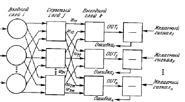
Rice. 3. Diagram of Rosenblatt's neural network.

Complications led to an increase in the number of adjustable parameters during training, but at the same time increased the ability to tune in to very complex patterns. Research in this area is now going in two closely related areas - both various network topologies and various tuning methods are being studied.

Neural networks are currently not only a tool for solving pattern recognition problems, but have been used in research on associative memory and image compression. Although this line of research overlaps strongly with the problems of pattern recognition, it is a separate section of cybernetics. For the recognizer at the moment, neural networks are nothing more than a very specific, parametrically defined set of mappings, which in this sense does not have any significant advantages over many other similar learning models that will be briefly listed below.

In connection with this assessment of the role of neural networks for proper recognition (that is, not for bionics, for which they are of paramount importance now), I would like to note the following: neural networks, being an extremely complex object for mathematical analysis, with their proper use, allow us to find very non-trivial laws in the data. Their difficulty for analysis, in the general case, is explained by their complex structure and, as a result, practically inexhaustible possibilities for generalizing a wide variety of regularities. But these advantages, as often happens, are a source of potential errors, the possibility of retraining. As will be discussed later, such a twofold view of the prospects of any learning model is one of the principles of machine learning.

Another popular direction in recognition is logical rules and decision trees. In comparison with the above-mentioned recognition methods, these methods most actively use the idea of ​​expressing our knowledge about the subject area in the form of probably the most natural (on a conscious level) structures - logical rules. An elementary logical rule means a statement like “if unclassified features are in the ratio X, then the classified ones are in the ratio Y”. An example of such a rule in medical diagnostics is the following: if the patient's age is over 60 years old and he has previously had a heart attack, then do not perform the operation - the risk of a negative outcome is high.

To search for logical rules in the data, 2 things are needed: to determine the measure of the “informativeness” of the rule and the space of rules. And the task of finding rules after that turns into a task of complete or partial enumeration in the space of rules in order to find the most informative of them. The definition of informativeness can be introduced in a variety of ways, and we will not dwell on this, considering that this is also some parameter of the model. The search space is defined in the standard way.

After finding sufficiently informative rules, the phase of “assembling” the rules into the final classifier begins. Without discussing in depth the problems that arise here (and there are a considerable number of them), we list 2 main methods of “assembly”. The first type is a linear list. The second type is weighted voting, when a certain weight is assigned to each rule, and the object is assigned by the classifier to the class for which the largest number of rules voted.

In fact, the rule building phase and the "assembly" phase are performed together and, when building a weighted vote or list, the search for rules on parts of the case data is called again and again to ensure a better fit between the data and the model.