- introductory lesson is free;
- A large number of experienced teachers (native and Russian-speaking);
- Courses NOT for a specific period (month, six months, year), but for a specific number of lessons (5, 10, 20, 50);
- Over 10,000 satisfied customers.
- The cost of one lesson with a Russian-speaking teacher - from 600 rubles, with a native speaker - from 1500 rubles
The concept of a variation series. The first step in systematizing the materials of statistical observation is counting the number of units that have one or another feature. Having arranged the units in ascending or descending order of their quantitative attribute and counting the number of units with a specific value of the attribute, we obtain a variation series. The variation series characterizes the distribution of units of a certain statistical population according to some quantitative attribute.
The variation series consists of two columns, the left column contains the values of the variable attribute, called variants and denoted by (x), and the right column contains absolute numbers showing how many times each variant occurs. The values in this column are called frequencies and are denoted by (f).
Schematically, the variation series can be represented in the form of Table 5.1:
Table 5.1
Type of variation series
|
Options (x) |
Frequencies (f) |
In the right column, relative indicators characterizing the proportion of the frequency of individual variants in the total amount of frequencies can also be used. These relative indicators are called frequencies and are conventionally denoted by , i.e. . The sum of all frequencies is equal to one. Frequencies can also be expressed as a percentage, and then their sum will be equal to 100%.
Variable signs can be of a different nature. Variants of some signs are expressed in integers, for example, the number of rooms in an apartment, the number of published books, etc. These signs are called discontinuous, or discrete. Variants of other features can take on any values within certain limits, such as the fulfillment of planned targets, wages, etc. These features are called continuous.
Discrete variation series. If the variants of the variational series are expressed as discrete values, then such a variational series is called discrete, its appearance is presented in Table. 5.2:
Table 5.2
Distribution of students by grades obtained in the exam
|
Ratings (x) |
Number of students (f) |
In % of total () |
The nature of the distribution in discrete series is depicted graphically as a distribution polygon, Fig.5.1.

Rice. 5.1. Distribution of students by grades obtained in the exam.
Interval variation series. For continuous features, variation series are constructed as interval series, i.e. feature values in them are expressed as intervals "from and to". In this case, the minimum value of a feature in such an interval is called the lower limit of the interval, and the maximum value is called the upper limit of the interval.
Interval variational series are built both for discontinuous features (discrete) and for those varying in a large range. Interval rows can be with equal and unequal intervals. In economic practice, for the most part, unequal intervals are used, progressively increasing or decreasing. Such a need arises especially in cases where the fluctuation of the sign is carried out unevenly and within large limits.
Consider the type of interval series with equal intervals, Table. 5.3:
Table 5.3
Distribution of workers by output
|
Output, tr. (X) |
Number of workers (f) |
Cumulative frequency (f´) |
The interval distribution series is graphically depicted as a histogram, Fig.5.2.

Fig.5.2. Distribution of workers by output
Accumulated (cumulative) frequency. In practice, there is a need to convert the distribution series into cumulative rows, built on the accumulated frequencies. They can be used to define structural averages that facilitate the analysis of distribution series data.
The cumulative frequencies are determined by successively adding to the frequencies (or frequencies) of the first group of these indicators of the subsequent groups of the distribution series. Cumulates and ogives are used to illustrate the distribution series. To build them, the values of a discrete feature (or the ends of the intervals) are marked on the abscissa axis, and the growing totals of frequencies (cumulate) are marked on the ordinate axis, Fig.5.3.

Rice. 5.3. The cumulative distribution of workers by development
If the scales of frequencies and variants are interchanged, i.e. reflect the accumulated frequencies on the abscissa axis, and the values of the options on the ordinate axis, then the curve characterizing the change in frequencies from group to group will be called the distribution ogive, Fig. 5.4.

Rice. 5.4. Ogiva distribution of workers for production
Variation series with equal intervals provide one of the most important requirements for statistical distribution series, ensuring their comparability in time and space.
Distribution density. However, the frequencies of individual unequal intervals in these series are not directly comparable. In such cases, to ensure the necessary comparability, the distribution density is calculated, i.e. determine how many units in each group are per unit of interval value.
When constructing a graph of the distribution of a variational series with unequal intervals, the height of the rectangles is determined in proportion not to the frequencies, but to the indicators of the distribution density of the values of the studied trait in the corresponding intervals.
Drawing up a variational series and its graphical representation is the first step in processing the initial data and the first step in analyzing the population under study. The next step in the analysis of variational series is the determination of the main generalizing indicators, called the characteristics of the series. These characteristics should give an idea of the average value of the attribute in the units of the population.
average value. The average value is a generalized characteristic of the studied trait in the studied population, reflecting its typical level per population unit in specific conditions of place and time.
The average value is always named, has the same dimension as the attribute of individual units of the population.
Before calculating the average values, it is necessary to group the units of the studied population, highlighting qualitatively homogeneous groups.
The average calculated for the population as a whole is called the general average, and for each group - group averages.
There are two types of averages: power (arithmetic average, harmonic average, geometric average, root mean quadratic); structural (mode, median, quartiles, deciles).
The choice of the average for the calculation depends on the purpose.
Types of power averages and methods for their calculation. In the practice of statistical processing of the collected material, various problems arise, the solution of which requires different averages.
Mathematical statistics derive various means from power mean formulas:
where is the average value; x - individual options (feature values); z - exponent (at z = 1 - arithmetic mean, z = 0 geometric mean, z = - 1 - harmonic mean, z = 2 - mean quadratic).
However, the question of what type of average should be applied in each individual case is resolved by a specific analysis of the population under study.
The most common type of average in statistics is arithmetic mean. It is calculated in those cases when the volume of the averaged attribute is formed as the sum of its values for individual units of the studied statistical population.
Depending on the nature of the initial data, the arithmetic mean is determined in various ways:
If the data is ungrouped, then the calculation is carried out according to the formula of a simple average value
Calculation of the arithmetic mean in a discrete series occurs according to the formula 3.4.
Calculation of the arithmetic mean in the interval series. In an interval variation series, where the middle of the interval is conditionally taken as the value of a feature in each group, the arithmetic mean may differ from the mean calculated from ungrouped data. Moreover, the larger the interval in groups, the greater the possible deviations of the average calculated from the grouped data from the average calculated from the ungrouped data.
When calculating the average for an interval variation series, in order to perform the necessary calculations, one passes from the intervals to their midpoints. And then calculate the average value by the formula of the arithmetic weighted average.
Properties of the arithmetic mean. The arithmetic mean has some properties that allow us to simplify calculations, let's consider them.
1. The arithmetic mean of the constant numbers is equal to this constant number.
If x = a. Then  .
.
2. If the weights of all options are proportionally changed, i.e. increase or decrease by the same number of times, then the arithmetic mean of the new series will not change from this.
If all weights f are reduced by k times, then  .
.
3. The sum of positive and negative deviations of individual options from the average, multiplied by the weights, is equal to zero, i.e. ![]()
If , then . From here.
If all options are reduced or increased by some number, then the arithmetic mean of the new series will decrease or increase by the same amount.
Reduce all options x on the a, i.e. x´ = x– a.
Then 
The arithmetic mean of the initial series can be obtained by adding to the reduced mean the number previously subtracted from the variants a, i.e. .
5. If all options are reduced or increased in k times, then the arithmetic mean of the new series will decrease or increase by the same amount, i.e. in k once.
Let then  .
.
Hence , i.e. to obtain the average of the original series, the arithmetic mean of the new series (with reduced options) must be increased by k once.
Average harmonic. The harmonic mean is the reciprocal of the arithmetic mean. It is used when statistical information does not contain frequencies for individual population options, but is presented as their product (M = xf). The harmonic mean will be calculated using formula 3.5
|
|

The practical application of the harmonic mean is to calculate some indices, in particular, the price index.
Geometric mean. When using the geometric mean, the individual values of the attribute are, as a rule, relative values of the dynamics, built in the form of chain values, as a ratio to the previous level of each level in the dynamics series. The average thus characterizes the average growth rate.
The geometric mean is also used to determine the equidistant value from the maximum and minimum values of the attribute. For example, an insurance company enters into contracts for the provision of auto insurance services. Depending on the specific insured event, the insurance payment may vary from 10,000 to 100,000 dollars per year. The average insurance payout is US$.
The geometric mean is the value used as the average of the ratios or in the distribution series, presented as a geometric progression, when z = 0. This average is convenient to use when attention is paid not to absolute differences, but to the ratios of two numbers.
Formulas for calculation are as follows
where are variants of the averaged feature; - the product of options; f– frequency of options.
The geometric mean is used in calculating average annual growth rates.
Mean square. The root mean square formula is used to measure the degree of fluctuation of the individual values of a trait around the arithmetic mean in the distribution series. So, when calculating the indicators of variation, the average is calculated from the squares of the deviations of the individual values of the trait from the arithmetic mean.
The mean square value is calculated by the formula
|
|

In economic research, the modified form of the root mean square is widely used in the calculation of indicators of the variation of a trait, such as variance, standard deviation.
Majority rule. There is the following relationship between power-law averages - the larger the exponent, the greater the value of the average, Table 5.4:
Table 5.4
Relationship between averages
|
z value |
||||
|
The ratio between the averages |
This relation is called the rule of majorance.
Structural averages. To characterize the structure of the population, special indicators are used, which can be called structural averages. These measures include mode, median, quartiles, and deciles.
Fashion. Mode (Mo) is the most frequently occurring value of a feature in population units. Mode is the value of the feature that corresponds to the maximum point of the theoretical distribution curve.
Fashion is widely used in commercial practice in the study of consumer demand (when determining the sizes of clothes and shoes that are in great demand), price registration. There can be several mods in total.
Mode calculation in a discrete series. In a discrete series, the mode is the variant with the highest frequency. Consider finding a mode in a discrete series.
Calculation of fashion in an interval series. In the interval variation series, the central variant of the modal interval is approximately considered to be a mode, i.e. the interval that has the highest frequency (frequency). Within the interval, it is necessary to find the value of the attribute, which is the mode. For an interval series, the mode will be determined by the formula
|
|

where is the lower limit of the modal interval; is the value of the modal interval; is the frequency corresponding to the modal interval; is the frequency preceding the modal interval; is the frequency of the interval following the modal.
Median. The median () is the value of the feature in the middle unit of the ranked series. A ranked series is a series in which the characteristic values are written in ascending or descending order. Or the median is a value that divides the number of an ordered variational series into two equal parts: one part has a value of a variable feature that is less than the average variant, and the other is large.
To find the median, its serial number is first determined. To do this, with an odd number of units, one is added to the sum of all frequencies and everything is divided by two. With an even number of units, the median is found as the value of the attribute of the unit, the serial number of which is determined by the total sum of frequencies divided by two. Knowing the ordinal number of the median, it is easy to find its value from the accumulated frequencies.
Calculation of the median in a discrete series. According to the sample survey, data were obtained on the distribution of families by the number of children, Table. 5.5. To determine the median, first determine its ordinal number
= ![]()
Then we build a series of accumulated frequencies (, by the serial number and the accumulated frequency we find the median. The accumulated frequency 33 shows that in 33 families the number of children does not exceed 1 child, but since the number of the median is 50, the median will be in the range from 34 to 55 families.
Table 5.5
Distribution of the number of families from the number of children
|
Number of children in the family |
The number of families, is the value of the median interval; All considered forms of the power mean have an important property (in contrast to structural means) – the formula for determining the mean includes all values of the series i.e. the size of the average is influenced by the value of each option. On the one hand, this is a very positive property. in this case, the effect of all causes affecting all units of the population under study is taken into account. On the other hand, even one observation that was accidentally included in the initial data can significantly distort the idea of the level of development of the studied trait in the population under consideration (especially in short series). Quartiles and deciles. By analogy with finding the median in variational series, one can find the value of a feature in any ranked series unit in order. So, in particular, one can find the value of a feature for units dividing the series into 4 equal parts, into 10, etc. Quartiles. Variants that divide the ranked series into four equal parts are called quartiles. At the same time, the following are distinguished: the lower (or first) quartile (Q1) - the value of the feature at the unit of the ranked series, dividing the population in the ratio of ¼ to ¾ and the upper (or third) quartile (Q3) - the value of the feature at the unit of the ranked series, dividing the population in the ratio ¾ to ¼. The second quartile is the median Q2 = Me. The lower and upper quartiles in the interval series are calculated using the formula similar to the median. where is the lower limit of the interval containing the lower and upper quartiles, respectively; is the cumulative frequency of the interval preceding the interval containing the lower or upper quartile; – frequencies of quartile intervals (lower and upper) The intervals containing Q1 and Q3 are determined from the accumulated frequencies (or frequencies). Deciles. In addition to quartiles, deciles are calculated - options that divide the ranked series into 10 equal parts. They are denoted by D, the first decile D1 divides the series in the ratio of 1/10 and 9/10, the second D2 - 2/10 and 8/10, etc. They are calculated in the same way as the median and quartiles. Both the median, and quartiles, and deciles belong to the so-called ordinal statistics, which is understood as a variant that occupies a certain ordinal place in a ranked series. |
The grouping method also allows you to measure variation(variability, fluctuation) of signs. With a relatively small number of population units, the variation is measured on the basis of a ranked series of units that make up the population. The row is called ranked if the units are arranged in ascending (descending) feature.
However, ranked series are rather indicative when a comparative characteristic of variation is needed. In addition, in many cases one has to deal with statistical aggregates consisting of a large number of units, which are practically difficult to represent in the form of a specific series. In this regard, for the initial general acquaintance with statistical data and especially to facilitate the study of the variation of signs, the studied phenomena and processes are usually combined into groups, and the results of the grouping are drawn up in the form of group tables.
If there are only two columns in the group table - groups according to the selected feature (options) and the number of groups (frequencies or frequencies), it is called near distribution.
Distribution range - the simplest type of structural grouping according to one attribute, displayed in a group table with two columns containing variants and frequencies of the attribute. In many cases, with such a structural grouping, i.e. with the compilation of distribution series, the study of the initial statistical material begins.
A structural grouping in the form of a distribution series can be turned into a true structural grouping if the selected groups are characterized not only by frequencies, but also by other statistical indicators. The main purpose of distribution series is to study the variation of features. The theory of distribution series is developed in detail by mathematical statistics.
The distribution series are divided into attributive(grouping by attributive characteristics, for example, the division of the population by sex, nationality, marital status, etc.) and variational(grouping by quantitative characteristics).
Variation series is a group table that contains two columns: a grouping of units according to one quantitative attribute and the number of units in each group. The intervals in the variation series are usually formed equal and closed. The variation series is the following grouping of the Russian population in terms of average per capita cash income (Table 3.10).
Table 3.10
Distribution of Russia's population by average per capita income in 2004-2009
|
Population groups by average per capita cash income, rub./month |
Population in the group, in % of the total |
|||||
|
8 000,1-10 000,0 |
||||||
|
10 000,1-15 000,0 |
||||||
|
15 000,1-25 000,0 |
||||||
|
Over 25,000.0 |
||||||
|
All population |
||||||
Variational series, in turn, are divided into discrete and interval. Discrete variation series combine variants of discrete features that vary within narrow limits. An example of a discrete variation series is the distribution of Russian families according to the number of children they have.
Interval variational series combine variants of either continuous features or discrete features that change over a wide range. The interval series is the variational series of the distribution of the Russian population in terms of average per capita cash income.
Discrete variational series are not used very often in practice. Meanwhile, compiling them is not difficult, since the composition of the groups is determined by the specific variants that the studied grouping characteristics actually possess.
Interval variational series are more widespread. In compiling them, the difficult question arises of the number of groups, as well as the size of the intervals that should be established.
The principles for resolving this issue are set out in the chapter on the methodology for constructing statistical groupings (see paragraph 3.3).
Variation series are a means of collapsing or compressing diverse information into a compact form; they can be used to make a fairly clear judgment about the nature of the variation, to study the differences in the signs of the phenomena included in the set under study. But the most important significance of the variational series is that on their basis the special generalizing characteristics of the variation are calculated (see Chapter 7).
Variation series: definition, types, main characteristics. Method of calculation
fashion, median, arithmetic mean in medical and statistical studies
(Show on a conditional example).
A variational series is a series of numerical values of the trait under study, which differ from each other in their magnitude and are arranged in a certain sequence (in ascending or descending order). Each numerical value of the series is called a variant (V), and the numbers showing how often this or that variant occurs in the composition of this series is called the frequency (p).
The total number of cases of observations, of which the variation series consists, is denoted by the letter n. The difference in the meaning of the studied characteristics is called variation. If the variable sign does not have a quantitative measure, the variation is called qualitative, and the distribution series is called attributive (for example, distribution by disease outcome, health status, etc.).
If a variable sign has a quantitative expression, such a variation is called quantitative, and the distribution series is called variational.
Variational series are divided into discontinuous and continuous - according to the nature of the quantitative trait, simple and weighted - according to the frequency of occurrence of the variant.
In a simple variational series, each variant occurs only once (p=1), in a weighted one, the same variant occurs several times (p>1). Examples of such series will be discussed later in the text. If the quantitative attribute is continuous, i.e. between integer values there are intermediate fractional values, the variational series is called continuous.
For example: 10.0 - 11.9
14.0 - 15.9, etc.
If the quantitative sign is discontinuous, i.e. its individual values (options) differ from each other by an integer and do not have intermediate fractional values, the variation series is called discontinuous or discrete.
Using the data from the previous example about the heart rate
for 21 students, we will build a variation series (Table 1).
Table 1
Distribution of medical students by pulse rate (bpm)
Thus, to build a variational series means to systematize, streamline the existing numerical values (options), i.e. arrange in a certain sequence (in ascending or descending order) with their corresponding frequencies. In the example under consideration, the options are arranged in ascending order and are expressed as discontinuous (discrete) integers, each option occurs several times, i.e. we are dealing with a weighted, discontinuous or discrete variational series.
As a rule, if the number of observations in the statistical population we are studying does not exceed 30, then it is enough to arrange all the values of the trait under study in a variational series in increasing order, as in Table. 1, or in descending order.
With a large number of observations (n>30), the number of occurring variants can be very large, in this case an interval or grouped variational series is compiled, in which, to simplify subsequent processing and clarify the nature of the distribution, the variants are combined into groups.
Usually the number of group options ranges from 8 to 15.
There must be at least 5 of them, because. otherwise, it will be too rough, excessive enlargement, which distorts the overall picture of variation and greatly affects the accuracy of the average values. When the number of group options is more than 20-25, the accuracy of calculating the average values increases, but the features of the variation of the attribute are significantly distorted and mathematical processing becomes more complicated.
When compiling a grouped series, it is necessary to take into account
− variant groups must be placed in a specific order (ascending or descending);
- the intervals in the variant groups should be the same;
− the values of the boundaries of the intervals should not coincide, because it will not be clear in which groups to attribute individual options;
- it is necessary to take into account the qualitative features of the collected material when setting the limits of the intervals (for example, when studying the weight of adults, an interval of 3-4 kg is acceptable, and for children in the first months of life it should not exceed 100 g.)
Let's build a grouped (interval) series that characterizes the data on the pulse rate (number of beats per minute) for 55 medical students before the exam: 64, 66, 60, 62,
64, 68, 70, 66, 70, 68, 62, 68, 70, 72, 60, 70, 74, 62, 70, 72, 72,
64, 70, 72, 76, 76, 68, 70, 58, 76, 74, 76, 76, 82, 76, 72, 76, 74,
79, 78, 74, 78, 74, 78, 74, 74, 78, 76, 78, 76, 80, 80, 80, 78, 78.
To build a grouped series, you need:
1. Determine the value of the interval;
2. Determine the middle, beginning and end of the groups of the variant of the variation series.
● The value of the interval (i) is determined by the number of expected groups (r), the number of which is set depending on the number of observations (n) according to a special table
Number of groups depending on the number of observations:
In our case, for 55 students, it is possible to make up from 8 to 10 groups.
The value of the interval (i) is determined by the following formula -
i = Vmax-Vmin/r
In our example, the value of the interval is 82-58/8= 3.
If the interval value is a fractional number, the result should be rounded up to an integer.
There are several types of averages:
● arithmetic mean,
● geometric mean,
● harmonic mean,
● root mean square,
● medium progressive,
● median
In medical statistics, arithmetic averages are most often used.
The arithmetic mean (M) is a generalizing value that determines the typical value that is characteristic of the entire population. The main methods for calculating M are: the arithmetic mean method and the method of moments (conditional deviations).
The arithmetic mean method is used to calculate the simple arithmetic mean and the weighted arithmetic mean. The choice of method for calculating the arithmetic mean value depends on the type of variation series. In the case of a simple variational series, in which each variant occurs only once, the simple arithmetic mean is determined by the formula:
where: М – arithmetic mean value;
V is the value of the variable feature (options);
Σ - indicates the action - summation;
n is the total number of observations.
An example of calculating the arithmetic mean is simple. Respiratory rate (number of breaths per minute) in 9 men aged 35: 20, 22, 19, 15, 16, 21, 17, 23, 18.
To determine the average level of respiratory rate in men aged 35, it is necessary:
1. Build a variational series by placing all options in ascending or descending order. We have obtained a simple variational series, because variant values occur only once.
M = ∑V/n = 171/9 = 19 breaths per minute
Output. The respiratory rate in men aged 35 is on average 19 breaths per minute.
If individual values of a variant are repeated, there is no need to write out each variant in a line; it is enough to list the sizes of the variant that occur (V) and next to indicate the number of their repetitions (p). such a variational series, in which the variants are, as it were, weighted according to the number of frequencies corresponding to them, is called the weighted variational series, and the calculated average value is the arithmetic weighted average.
The arithmetic weighted average is determined by the formula: M= ∑Vp/n
where n is the number of observations equal to the sum of frequencies - Σр.
An example of calculating the arithmetic weighted average.
The duration of disability (in days) in 35 patients with acute respiratory diseases (ARI) treated by a local doctor during the first quarter of the current year was: 6, 7, 5, 3, 9, 8, 7, 5, 6, 4, 9, 8, 7, 6, 6, 9, 6, 5, 10, 8, 7, 11, 13, 5, 6, 7, 12, 4, 3, 5, 2, 5, 6, 6, 7 days .
The methodology for determining the average duration of disability in patients with acute respiratory infections is as follows:
1. Let's build a weighted variational series, because individual variant values are repeated several times. To do this, you can arrange all the options in ascending or descending order with their corresponding frequencies.
In our case, the options are in ascending order.
2. Calculate the arithmetic weighted average using the formula: M = ∑Vp/n = 233/35 = 6.7 days
Distribution of patients with acute respiratory infections by duration of disability:
| Duration of incapacity for work (V) | Number of patients (p) | vp |
| ∑p = n = 35 | ∑Vp = 233 |
Output. The duration of disability in patients with acute respiratory diseases averaged 6.7 days.
Mode (Mo) is the most common variant in the variation series. For the distribution presented in the table, the mode corresponds to the variant equal to 10, it occurs more often than others - 6 times.
Distribution of patients by length of stay in a hospital bed (in days)
| V |
| p |
Sometimes it is difficult to determine the exact value of the mode, since there may be several observations in the data being studied that occur “most often”.
Median (Me) is a non-parametric indicator that divides the variation series into two equal halves: the same number of options is located on both sides of the median.
For example, for the distribution shown in the table, the median is 10 because on both sides of this value is located on the 14th option, i.e. the number 10 occupies a central position in this series and is its median.
Given that the number of observations in this example is even (n=34), the median can be determined as follows:
Me = 2+3+4+5+6+5+4+3+2/2 = 34/2 = 17
This means that the middle of the series falls on the seventeenth option, which corresponds to a median of 10. For the distribution presented in the table, the arithmetic mean is:
M = ∑Vp/n = 334/34 = 10.1
So, for 34 observations from Table. 8, we got: Mo=10, Me=10, arithmetic mean (M) is 10.1. In our example, all three indicators turned out to be equal or close to each other, although they are completely different.
The arithmetic mean is the resultant sum of all influences; all options, without exception, take part in its formation, including extreme ones, often atypical for a given phenomenon or set.
Mode and median, in contrast to the arithmetic mean, do not depend on the value of all individual values of the variable attribute (the values of the extreme variants and the degree of scattering of the series). The arithmetic mean characterizes the entire mass of observations, the mode and median characterize the bulk
Statistical distribution series- this is an ordered distribution of population units into groups according to a certain varying attribute.Depending on the trait underlying the formation of a distribution series, there are attribute and variation distribution series.
The presence of a common feature is the basis for the formation of a statistical population, which is the results of a description or measurement of common features of the objects of study.
The subject of study in statistics are changing (varying) features or statistical features.
Types of statistical features.
Distribution series are called attribute series. built on quality grounds. Attributive- this is a sign that has a name (for example, a profession: a seamstress, teacher, etc.).
It is customary to arrange the distribution series in the form of tables. In table. 2.8 shows an attribute series of distribution.
Table 2.8 - Distribution of types of legal assistance provided by lawyers to citizens of one of the regions of the Russian Federation.
Variation series are distribution series built on a quantitative basis. Any variational series consists of two elements: variants and frequencies.
Variants are individual values of a feature that it takes in a variation series.
Frequencies are the numbers of individual variants or each group of the variation series, i.e. these are numbers showing how often certain options occur in a distribution series. The sum of all frequencies determines the size of the entire population, its volume.
Frequencies are called frequencies, expressed in fractions of a unit or as a percentage of the total. Accordingly, the sum of the frequencies is equal to 1 or 100%. The variational series allows us to evaluate the form of the distribution law based on actual data.
Depending on the nature of the variation of the trait, there are discrete and interval variation series.
An example of a discrete variational series is given in Table. 2.9.
Table 2.9 - Distribution of families by the number of rooms occupied in individual apartments in 1989 in the Russian Federation.
Variation series
In the general population, a certain quantitative trait is being investigated. A sample of volume is randomly extracted from it n, that is, the number of elements in the sample is n. At the first stage of statistical processing, ranging samples, i.e. number ordering x 1 , x 2 , …, x n Ascending. Each observed value x i called option. Frequency m i is the number of observations of the value x i in the sample. Relative frequency (frequency) w i is the frequency ratio m i to sample size n: .When studying a variational series, the concepts of cumulative frequency and cumulative frequency are also used. Let be x some number. Then the number of options , whose values are less x, is called the accumulated frequency: for x i
An attribute is called discretely variable if its individual values (variants) differ from each other by some finite amount (usually an integer). A variational series of such a feature is called a discrete variational series.
Table 1. General view of the discrete variational series of frequencies
| Feature values | x i | x 1 | x2 | … | x n |
| Frequencies | m i | m 1 | m2 | … | m n |
An attribute is called continuously varying if its values differ from each other by an arbitrarily small amount, i.e. the sign can take any value in a certain interval. A continuous variation series for such a trait is called an interval series.
Table 2. General view of the interval variation series of frequencies
Table 3. Graphic images of the variation series
| Row | Polygon or histogram | Empirical distribution function | |
| Discrete |  |  | 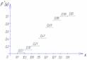 |
| interval |  | 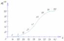 |  |
For graphic representation of variational series, polygon, histogram, cumulative curve and empirical distribution function are most often used.
In table. 2.3 (Grouping of the population of Russia according to the size of the average per capita income in April 1994) is presented interval variation series.
It is convenient to analyze the distribution series using a graphical representation, which also makes it possible to judge the shape of the distribution. A visual representation of the nature of the change in the frequencies of the variational series is given by polygon and histogram.
The polygon is used when displaying discrete variational series.
Let us depict, for example, graphically the distribution of housing stock by type of apartments (Table 2.10).
Table 2.10 - Distribution of the housing stock of the urban area by type of apartments (conditional figures).

Rice. Housing distribution polygon
On the y-axis, not only the values of frequencies, but also the frequencies of the variation series can be plotted.
The histogram is taken to display the interval variation series. When constructing a histogram, the values of the intervals are plotted on the abscissa axis, and the frequencies are depicted by rectangles built on the corresponding intervals. The height of the columns in the case of equal intervals should be proportional to the frequencies. A histogram is a graph in which a series is shown as bars adjacent to each other.
Let's graphically depict the interval distribution series given in Table. 2.11.
Table 2.11 - Distribution of families by the size of living space per person (conditional figures).
| N p / p | Groups of families by the size of living space per person | Number of families with a given size of living space | Accumulated number of families |
| 1 | 3 – 5 | 10 | 10 |
| 2 | 5 – 7 | 20 | 30 |
| 3 | 7 – 9 | 40 | 70 |
| 4 | 9 – 11 | 30 | 100 |
| 5 | 11 – 13 | 15 | 115 |
| TOTAL | 115 | ---- | |

Rice. 2.2. Histogram of the distribution of families by the size of living space per person
Using the data of the accumulated series (Table 2.11), we construct distribution cumulative.

Rice. 2.3. The cumulative distribution of families by the size of living space per person
The representation of a variational series in the form of a cumulate is especially effective for variational series, the frequencies of which are expressed as fractions or percentages of the sum of the frequencies of the series.
If we change the axes in the graphic representation of the variational series in the form of a cumulate, then we get ogivu. On fig. 2.4 shows an ogive built on the basis of the data in Table. 2.11.
A histogram can be converted to a distribution polygon by finding the midpoints of the sides of the rectangles and then connecting these points with straight lines. The resulting distribution polygon is shown in fig. 2.2 dotted line.
When constructing a histogram of the distribution of a variational series with unequal intervals, along the ordinate axis, not frequencies are applied, but the distribution density of the feature in the corresponding intervals.
The distribution density is the frequency calculated per unit interval width, i.e. how many units in each group are per unit interval value. An example of calculating the distribution density is presented in Table. 2.12.
Table 2.12 - Distribution of enterprises by the number of employees (figures are conditional)
| N p / p | Groups of enterprises by the number of employees, pers. | Number of enterprises | Interval size, pers. | Distribution density |
| BUT | 1 | 2 | 3=1/2 | |
| 1 | up to 20 | 15 | 20 | 0,75 |
| 2 | 20 – 80 | 27 | 60 | 0,25 |
| 3 | 80 – 150 | 35 | 70 | 0,5 |
| 4 | 150 – 300 | 60 | 150 | 0,4 |
| 5 | 300 – 500 | 10 | 200 | 0,05 |
| TOTAL | 147 | ---- | ---- |
For a graphical representation of variation series can also be used cumulative curve. With the help of the cumulate (the curve of the sums), a series of accumulated frequencies is displayed. Accumulated frequencies are determined by sequentially summing the frequencies by groups and show how many units of the population have feature values no greater than the considered value.

Rice. 2.4. Ogiva distribution of families according to the size of living space per person
When constructing the cumulate of an interval variation series, the variants of the series are plotted along the abscissa axis, and the accumulated frequencies along the ordinate axis.
Continuous variation series
A continuous variational series is a series built on the basis of a quantitative statistical sign. Example. The average duration of diseases of convicts (days per person) in the autumn-winter period in the current year was:| 7,0 | 6,0 | 5,9 | 9,4 | 6,5 | 7,3 | 7,6 | 9,3 | 5,8 | 7,2 |
| 7,1 | 8,3 | 7,5 | 6,8 | 7,1 | 9,2 | 6,1 | 8,5 | 7,4 | 7,8 |
| 10,2 | 9,4 | 8,8 | 8,3 | 7,9 | 9,2 | 8,9 | 9,0 | 8,7 | 8,5 |
variational called distribution series built on a quantitative basis. The values of quantitative characteristics in individual units of the population are not constant, more or less differ from each other.
Variation- fluctuation, variability of the value of the attribute in units of the population. Separate numerical values of the trait occurring in the studied population are called options values. The insufficiency of the average value for a complete characterization of the population makes it necessary to supplement the average values with indicators that make it possible to assess the typicality of these averages by measuring the fluctuation (variation) of the trait under study.
The presence of variation is due to the influence of a large number of factors on the formation of the trait level. These factors act with unequal force and in different directions. Variation indicators are used to describe the measure of trait variability.
Tasks of the statistical study of variation:
- 1) the study of the nature and degree of variation of signs in individual units of the population;
- 2) determination of the role of individual factors or their groups in the variation of certain features of the population.
In statistics, special methods for studying variation are used, based on the use of a system of indicators, from by which variation is measured.
The study of variation is essential. The measurement of variations is necessary when conducting sample observation, correlation and variance analysis, etc. Ermolaev O.Yu. Mathematical statistics for psychologists: Textbook [Text] / O.Yu. Ermolaev. - M.: Flint Publishing House of the Moscow Psychological and Social Institute, 2012. - 335p.
According to the degree of variation, one can judge the homogeneity of the population, the stability of individual values of features and the typicality of the average. On their basis, indicators of the closeness of the relationship between the signs, indicators for assessing the accuracy of selective observation are developed.
There is variation in space and variation in time.
Variation in space is understood as the fluctuation of the values of a feature in units of the population representing separate territories. Under the variation in time is meant the change in the values of the attribute in different periods of time.
To study the variation in the distribution series, all variants of the attribute values are arranged in ascending or descending order. This process is called series ranking.
The simplest signs of variation are minimum and maximum- the smallest and largest value of the attribute in the aggregate. The number of repetitions of individual variants of feature values is called the frequency of repetition (fi). It is convenient to replace frequencies with frequencies - wi. Frequency - a relative indicator of frequency, which can be expressed in fractions of a unit or a percentage and allows you to compare variation series with a different number of observations. Expressed by the formula:
where Xmax, Xmin - the maximum and minimum values of the attribute in the aggregate; n is the number of groups.
To measure the variation of a trait, various absolute and relative indicators are used. The absolute indicators of variation include the range of variation, the average linear deviation, variance, standard deviation. The relative indicators of fluctuation include the coefficient of oscillation, the relative linear deviation, the coefficient of variation.
An example of finding a variation series
The task. For this sample:
- a) Find a variation series;
- b) Construct the distribution function;
No.=42. Sample items:
1 5 1 8 1 3 9 4 7 3 7 8 7 3 2 3 5 3 8 3 5 2 8 3 7 9 5 8 8 1 2 2 5 1 6 1 7 6 7 7 6 2
Solution.
- a) construction of a ranked variational series:
- 1 1 1 1 1 1 2 2 2 2 2 3 3 3 3 3 3 3 4 5 5 5 5 5 6 6 6 7 7 7 7 7 7 7 8 8 8 8 8 8 9 9
- b) construction of a discrete variational series.
Let's calculate the number of groups in the variation series using the Sturgess formula:
Let's take the number of groups equal to 7.
Knowing the number of groups, we calculate the value of the interval:
For the convenience of constructing the table, we will take the number of groups equal to 8, the interval will be 1.
Rice. one The volume of sales of goods by the store for a certain period of time
