The most common form of statistical indicators used in socio-economic research is the average value, which is a generalized quantitative characteristic of a sign of a statistical population. Average values are, as it were, "representatives" of the entire series of observations. In many cases, the average can be determined through the initial ratio of the average (ISS) or its logical formula: . So, for example, to calculate the average wages of employees of an enterprise, it is necessary to divide the total wage fund by the number of employees: The numerator of the initial ratio of the average is its defining indicator. For the average wage, such a determining indicator is the wage fund. For each indicator used in the socio-economic analysis, only one true reference ratio can be compiled to calculate the average. It should also be added that in order to more accurately estimate the standard deviation for small samples (with the number of elements less than 30), the denominator of the expression under the root should not use n, a n- 1.
The concept and types of averages
Average value- this is a generalizing indicator of the statistical population, which extinguishes individual differences in the values of statistical quantities, allowing you to compare different populations with each other. Exist 2 classes average values: power and structural. Structural averages are fashion and median , but the most commonly used power averages various kinds.Power averages
Power averages can be simple and weighted.
A simple average is calculated when there are two or more ungrouped statistical values, arranged in an arbitrary order according to the following general formula of the average power law (for different values of k (m)):
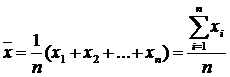
The weighted average is calculated from the grouped statistics using the following general formula:

Where x - the average value of the phenomenon under study; x i – i-th variant of the averaged feature ;
f i is the weight of the i-th option.

Where X are the values of individual statistical values or the midpoints of grouping intervals;
m - exponent, on the value of which the following types of power averages depend:
at m = -1 harmonic mean;
for m = 0, the geometric mean;
for m = 1, the arithmetic mean;
at m = 2, the root mean square;
at m = 3, the average cubic.
Using the general formulas for simple and weighted averages with different exponents m, we obtain particular formulas of each type, which will be discussed in detail below.
Arithmetic mean
Arithmetic mean - the initial moment of the first order, the mathematical expectation of the values of a random variable with a large number of trials;
The arithmetic mean is the most commonly used average value, which is obtained by substituting m = 1 into the general formula. Arithmetic mean simple has the following form:
 or
or ![]()
Where X are the values of the quantities for which it is necessary to calculate the average value; N is the total number of X values (the number of units in the studied population).
For example, a student passed 4 exams and received the following grades: 3, 4, 4 and 5. Calculate the average score using the simple arithmetic mean formula: (3+4+4+5)/4 = 16/4 = 4. Arithmetic mean weighted has the following form:

Where f is the number of values with the same X value (frequency). >For example, a student passed 4 exams and received the following grades: 3, 4, 4 and 5. Calculate the average score using the arithmetic weighted average formula: (3*1 + 4*2 + 5*1)/4 = 16/4 = 4 . If the X values are given as intervals, then the midpoints of the X intervals are used for calculations, which are defined as half the sum of the upper and lower boundaries of the interval. And if the interval X does not have a lower or upper limit (open interval), then to find it, the range (the difference between the upper and lower limits) of the adjacent interval X is used. For example, at the enterprise there are 10 employees with work experience up to 3 years, 20 - with work experience from 3 to 5 years, 5 employees - with work experience of more than 5 years. Then we calculate the average length of service of employees using the arithmetic weighted average formula, taking as X the middle of the length of service intervals (2, 4 and 6 years): (2*10+4*20+6*5)/(10+20+5) = 3.71 years.
AVERAGE function
This function calculates the average (arithmetic) of its arguments.
AVERAGE(number1, number2, ...)
Number1, number2, ... are 1 to 30 arguments for which the average is calculated.
Arguments must be numbers or names, arrays or references containing numbers. If the argument, which is an array or a link, contains texts, booleans, or empty cells, then those values are ignored; however, cells that contain null values are counted.
AVERAGE function
Calculates the arithmetic mean of the values given in the argument list. In addition to numbers, text and logical values, such as TRUE and FALSE, can participate in the calculation.
AVERAGE(value1, value2,...)
Value1, value2,... are 1 to 30 cells, cell ranges, or values for which the average is calculated.
Arguments must be numbers, names, arrays, or references. Arrays and links containing text are interpreted as 0 (zero). Empty text ("") is interpreted as 0 (zero). Arguments containing the value TRUE are interpreted as 1, Arguments containing the value FALSE are interpreted as 0 (zero).
The arithmetic mean is used most often, but there are times when other types of averages are needed. Let's consider such cases further.
Average harmonic
Harmonic mean for determining the average sum of reciprocals;
Average harmonic is used when the original data do not contain frequencies f for individual values of X, but are presented as their product Xf. Denoting Xf=w, we express f=w/X, and substituting these notations into the weighted arithmetic mean formula, we obtain the weighted harmonic mean formula:
Thus, the harmonic weighted average is used when the frequencies f are unknown, but w=Xf is known. In cases where all w=1, that is, the individual values of X occur 1 time, the harmonic simple mean formula is applied:  or
or  For example, a car was traveling from point A to point B at a speed of 90 km/h and back at a speed of 110 km/h. To determine the average speed, we apply the harmonic simple formula, since the example gives the distance w 1 \u003d w 2 (the distance from point A to point B is the same as from B to A), which is equal to the product of speed (X) and time ( f). Average speed = (1+1)/(1/90+1/110) = 99 km/h.
SRHARM function
Returns the harmonic mean of the data set. The harmonic mean is the reciprocal of the arithmetic mean of reciprocals.
SGARM(number1, number2, ...)
Number1, number2, ... are 1 to 30 arguments for which the average is calculated. You can use an array or an array reference instead of semicolon-separated arguments.
The harmonic mean is always less than the geometric mean, which is always less than the arithmetic mean.
Geometric mean
Geometric mean for estimating the average growth rate of random variables, finding the value of a feature equidistant from the minimum and maximum values;
Geometric mean used in determining average relative changes. The geometric mean value gives the most accurate averaging result if the task is to find such a value of X, which would be equidistant from both the maximum and minimum values of X. For example, between 2005 and 2008inflation index in Russia was: in 2005 - 1.109; in 2006 - 1,090; in 2007 - 1,119; in 2008 - 1,133. Since the inflation index is a relative change (dynamic index), then you need to calculate the average value using the geometric mean: (1.109 * 1.090 * 1.119 * 1.133) ^ (1/4) = 1.1126, that is, for the period from 2005 to 2008 annually prices grew by an average of 11.26%. An erroneous calculation on the arithmetic mean would give an incorrect result of 11.28%.SRGEOM function
Returns the geometric mean of an array or range of positive numbers. For example, the CAGEOM function can be used to calculate the average growth rate if compound income with variable rates is given.
SRGEOM(number1; number2; ...)
Number1, number2, ... are 1 to 30 arguments for which the geometric mean is calculated. You can use an array or an array reference instead of semicolon-separated arguments.
root mean square
The root mean square is the initial moment of the second order.
root mean square is used when the initial values of X can be both positive and negative, for example, when calculating average deviations.Average cubic
The average cubic is the initial moment of the third order.
Average cubic is used extremely rarely, for example, when calculating poverty indices for developing countries (HPI-1) and for developed countries (HPI-2), proposed and calculated by the UN.In most cases, the data is concentrated around some central point. Thus, to describe any data set, it is enough to indicate the average value. Consider successively three numerical characteristics that are used to estimate the mean value of the distribution: arithmetic mean, median and mode.
Average
The arithmetic mean (often referred to simply as the mean) is the most common estimate of the mean of a distribution. It is the result of dividing the sum of all observed numerical values by their number. For a sample of numbers X 1, X 2, ..., Xn, the sample mean (denoted by the symbol ) equals \u003d (X 1 + X 2 + ... + Xn) / n, or
where is the sample mean, n- sample size, Xi– i-th element of the sample.
Download note in or format, examples in format
Consider calculating the arithmetic average of the five-year average annual returns of 15 very high-risk mutual funds (Figure 1).

Rice. 1. Average annual return on 15 very high-risk mutual funds
The sample mean is calculated as follows:

This is a good return, especially when compared to the 3-4% return that bank or credit union depositors received over the same time period. If you sort the return values, it is easy to see that eight funds have a return above, and seven - below the average. The arithmetic mean acts as a balance point, so that low-income funds balance out high-income funds. All elements of the sample are involved in the calculation of the average. None of the other estimators of the distribution mean have this property.
When to calculate the arithmetic mean. Since the arithmetic mean depends on all elements of the sample, the presence of extreme values significantly affects the result. In such situations, the arithmetic mean can distort the meaning of the numerical data. Therefore, when describing a data set containing extreme values, it is necessary to indicate the median or the arithmetic mean and the median. For example, if the return of the RS Emerging Growth fund is removed from the sample, the sample average of the return of the 14 funds decreases by almost 1% to 5.19%.
Median
The median is the middle value of an ordered array of numbers. If the array does not contain repeating numbers, then half of its elements will be less than and half more than the median. If the sample contains extreme values, it is better to use the median rather than the arithmetic mean to estimate the mean. To calculate the median of a sample, it must first be sorted.
This formula is ambiguous. Its result depends on whether the number is even or odd. n:
- If the sample contains an odd number of items, the median is (n+1)/2-th element.
- If the sample contains an even number of elements, the median lies between the two middle elements of the sample and is equal to the arithmetic mean calculated over these two elements.
To calculate the median for a sample of 15 very high-risk mutual funds, we first need to sort the raw data (Figure 2). Then the median will be opposite the number of the middle element of the sample; in our example number 8. Excel has a special function =MEDIAN() that works with unordered arrays too.

Rice. 2. Median 15 funds
Thus, the median is 6.5. This means that half of the very high-risk funds do not exceed 6.5, while the other half do so. Note that the median of 6.5 is slightly larger than the median of 6.08.
If we remove the profitability of the RS Emerging Growth fund from the sample, then the median of the remaining 14 funds will decrease to 6.2%, that is, not as significantly as the arithmetic mean (Fig. 3).

Rice. 3. Median 14 funds
Fashion
The term was first introduced by Pearson in 1894. Fashion is the number that occurs most often in the sample (the most fashionable). Fashion describes well, for example, the typical reaction of drivers to a traffic signal to stop traffic. A classic example of the use of fashion is the choice of the size of the produced batch of shoes or the color of the wallpaper. If a distribution has multiple modes, then it is said to be multimodal or multimodal (has two or more "peaks"). The multimodal distribution provides important information about the nature of the variable under study. For example, in sociological surveys, if a variable represents a preference or attitude towards something, then multimodality could mean that there are several distinctly different opinions. Multimodality is also an indicator that the sample is not homogeneous and that the observations may be generated by two or more "overlapped" distributions. Unlike the arithmetic mean, outliers do not affect the mode. For continuously distributed random variables, such as the average annual returns of mutual funds, the mode sometimes does not exist at all (or does not make sense). Since these indicators can take on a variety of values, repeating values are extremely rare.
Quartiles
Quartiles are measures that are most commonly used to evaluate the distribution of data when describing the properties of large numerical samples. While the median splits the ordered array in half (50% of the array elements are less than the median and 50% are greater), quartiles break the ordered dataset into four parts. The Q 1 , median and Q 3 values are the 25th, 50th and 75th percentile, respectively. The first quartile Q 1 is a number that divides the sample into two parts: 25% of the elements are less than, and 75% are more than the first quartile.
The third quartile Q 3 is a number that also divides the sample into two parts: 75% of the elements are less than, and 25% are more than the third quartile.
To calculate quartiles in versions of Excel prior to 2007, the function =QUARTILE(array, part) was used. Starting with Excel 2010, two functions apply:
- =QUARTILE.ON(array, part)
- =QUARTILE.EXC(array, part)
These two functions give slightly different values (Figure 4). For example, when calculating the quartiles for a sample containing data on the average annual return of 15 very high-risk mutual funds, Q 1 = 1.8 or -0.7 for QUARTILE.INC and QUARTILE.EXC, respectively. By the way, the QUARTILE function used earlier corresponds to the modern QUARTILE.ON function. To calculate quartiles in Excel using the above formulas, the data array can be left unordered.

Rice. 4. Calculate quartiles in Excel
Let's emphasize again. Excel can calculate quartiles for univariate discrete series, containing the values of a random variable. The calculation of quartiles for a frequency-based distribution is given in the section below.
geometric mean
Unlike the arithmetic mean, the geometric mean measures how much a variable has changed over time. The geometric mean is the root n th degree from the product n values (in Excel, the function = CUGEOM is used):
G= (X 1 * X 2 * ... * X n) 1/n
A similar parameter - the geometric mean of the rate of return - is determined by the formula:
G \u003d [(1 + R 1) * (1 + R 2) * ... * (1 + R n)] 1 / n - 1,
where R i- rate of return i-th period of time.
For example, suppose the initial investment is $100,000. By the end of the first year, it drops to $50,000, and by the end of the second year, it recovers to the original $100,000. The rate of return on this investment over a two-year period is equal to 0, since the initial and final amount of funds are equal to each other. However, the arithmetic average of annual rates of return is = (-0.5 + 1) / 2 = 0.25 or 25%, since the rate of return in the first year R 1 = (50,000 - 100,000) / 100,000 = -0.5 , and in the second R 2 = (100,000 - 50,000) / 50,000 = 1. At the same time, the geometric mean of the rate of return for two years is: G = [(1–0.5) * (1 + 1 )] 1/2 – 1 = ½ – 1 = 1 – 1 = 0. Thus, the geometric mean more accurately reflects the change (more precisely, no change) in the volume of investment over the biennium than the arithmetic mean.
Interesting Facts. First, the geometric mean will always be less than the arithmetic mean of the same numbers. Except for the case when all the taken numbers are equal to each other. Secondly, having considered the properties of a right triangle, one can understand why the mean is called geometric. The height of a right-angled triangle, lowered to the hypotenuse, is the average proportional between the projections of the legs on the hypotenuse, and each leg is the average proportional between the hypotenuse and its projection on the hypotenuse (Fig. 5). This gives a geometric way of constructing the geometric mean of two (lengths) segments: you need to build a circle on the sum of these two segments as a diameter, then the height, restored from the point of their connection to the intersection with the circle, will give the desired value:

Rice. 5. The geometric nature of the geometric mean (figure from Wikipedia)
The second important property of numerical data is their variation characterizing the degree of dispersion of the data. Two different samples can differ both in mean values and in variations. However, as shown in fig. 6 and 7, two samples can have the same variation but different means, or the same mean and completely different variation. The data corresponding to polygon B in Fig. 7 change much less than the data from which polygon A was built.

Rice. 6. Two symmetric bell-shaped distributions with the same spread and different mean values

Rice. 7. Two symmetric bell-shaped distributions with the same mean values and different scatter
There are five estimates of data variation:
- span,
- interquartile range,
- dispersion,
- standard deviation,
- the coefficient of variation.
scope
The range is the difference between the largest and smallest elements of the sample:
Swipe = XMax-XMin
The range of a sample containing data on the average annual returns of 15 very high-risk mutual funds can be calculated using an ordered array (see Figure 4): range = 18.5 - (-6.1) = 24.6. This means that the difference between the highest and lowest average annual returns for very high risk funds is 24.6%.
The range measures the overall spread of the data. Although the sample range is a very simple estimate of the total spread of the data, its weakness is that it does not take into account exactly how the data is distributed between the minimum and maximum elements. This effect is well seen in Fig. 8 which illustrates samples having the same range. The B scale shows that if the sample contains at least one extreme value, the sample range is a very inaccurate estimate of the scatter of the data.

Rice. 8. Comparison of three samples with the same range; the triangle symbolizes the support of the balance, and its location corresponds to the average value of the sample
Interquartile range
The interquartile, or mean, range is the difference between the third and first quartiles of the sample:
Interquartile range \u003d Q 3 - Q 1
This value makes it possible to estimate the spread of 50% of the elements and not to take into account the influence of extreme elements. The interquartile range for a sample containing data on the average annual returns of 15 very high-risk mutual funds can be calculated using the data in Fig. 4 (for example, for the function QUARTILE.EXC): Interquartile range = 9.8 - (-0.7) = 10.5. The interval between 9.8 and -0.7 is often referred to as the middle half.
It should be noted that the Q 1 and Q 3 values, and hence the interquartile range, do not depend on the presence of outliers, since their calculation does not take into account any value that would be less than Q 1 or greater than Q 3 . The total quantitative characteristics, such as the median, the first and third quartiles, and the interquartile range, which are not affected by outliers, are called robust indicators.
While the range and interquartile range provide an estimate of the total and mean scatter of the sample, respectively, neither of these estimates takes into account exactly how the data are distributed. Variance and standard deviation free from this shortcoming. These indicators allow you to assess the degree of fluctuation of the data around the mean. Sample variance is an approximation of the arithmetic mean calculated from the squared differences between each sample element and the sample mean. For a sample of X 1 , X 2 , ... X n the sample variance (denoted by the symbol S 2 is given by the following formula:

In general, the sample variance is the sum of the squared differences between the sample elements and the sample mean, divided by a value equal to the sample size minus one:

where - arithmetic mean, n- sample size, X i - i-th sample element X. In Excel before version 2007, the function =VAR() was used to calculate the sample variance, since version 2010, the function =VAR.V() is used.
The most practical and widely accepted estimate of data scatter is standard deviation. This indicator is denoted by the symbol S and is equal to the square root of the sample variance:

In Excel before version 2007, the =STDEV() function was used to calculate the standard deviation, from version 2010 the =STDEV.B() function is used. To calculate these functions, the data array can be unordered.
Neither the sample variance nor the sample standard deviation can be negative. The only situation in which the indicators S 2 and S can be zero is if all elements of the sample are equal. In this completely improbable case, the range and interquartile range are also zero.
Numeric data is inherently volatile. Any variable can take on many different values. For example, different mutual funds have different rates of return and loss. Due to the variability of numerical data, it is very important to study not only estimates of the mean, which are summative in nature, but also estimates of the variance, which characterize the scatter of the data.
The variance and standard deviation allow us to estimate the spread of data around the mean, in other words, to determine how many elements of the sample are less than the mean, and how many are greater. The dispersion has some valuable mathematical properties. However, its value is the square of a unit of measure - a square percentage, a square dollar, a square inch, etc. Therefore, a natural estimate of the variance is the standard deviation, which is expressed in the usual units of measurement - percent of income, dollars or inches.
The standard deviation allows you to estimate the amount of fluctuation of the sample elements around the mean value. In almost all situations, the majority of observed values lie within plus or minus one standard deviation from the mean. Therefore, knowing the arithmetic mean of the sample elements and the standard sample deviation, it is possible to determine the interval to which the bulk of the data belongs.
The standard deviation of returns on 15 very high-risk mutual funds is 6.6 (Figure 9). This means that the profitability of the bulk of funds differs from the average value by no more than 6.6% (i.e., it fluctuates in the range from – S= 6.2 – 6.6 = –0.4 to +S= 12.8). In fact, this interval contains a five-year average annual return of 53.3% (8 out of 15) of funds.

Rice. 9. Standard deviation
Note that in the process of summing the squared differences, items that are farther from the mean gain more weight than items that are closer. This property is the main reason why the arithmetic mean is most often used to estimate the mean of a distribution.
The coefficient of variation
Unlike previous scatter estimates, the coefficient of variation is a relative estimate. It is always measured as a percentage, not in the original data units. The coefficient of variation, denoted by the symbols CV, measures the scatter of the data around the mean. The coefficient of variation is equal to the standard deviation divided by the arithmetic mean and multiplied by 100%:

where S- standard sample deviation, - sample mean.
The coefficient of variation allows you to compare two samples, the elements of which are expressed in different units of measurement. For example, the manager of a mail delivery service intends to upgrade the fleet of trucks. When loading packages, there are two types of restrictions to consider: the weight (in pounds) and the volume (in cubic feet) of each package. Assume that in a sample of 200 bags, the average weight is 26.0 pounds, the standard deviation of the weight is 3.9 pounds, the average package volume is 8.8 cubic feet, and the standard deviation of the volume is 2.2 cubic feet. How to compare the spread of weight and volume of packages?
Since the units of measurement for weight and volume differ from each other, the manager must compare the relative spread of these values. The weight variation coefficient is CV W = 3.9 / 26.0 * 100% = 15%, and the volume variation coefficient CV V = 2.2 / 8.8 * 100% = 25% . Thus, the relative scatter of packet volumes is much larger than the relative scatter of their weights.
Distribution form
The third important property of the sample is the form of its distribution. This distribution can be symmetrical or asymmetric. To describe the shape of a distribution, it is necessary to calculate its mean and median. If these two measures are the same, the variable is said to be symmetrically distributed. If the mean value of a variable is greater than the median, its distribution has a positive skewness (Fig. 10). If the median is greater than the mean, the distribution of the variable is negatively skewed. Positive skewness occurs when the mean increases to unusually high values. Negative skewness occurs when the mean decreases to unusually small values. A variable is symmetrically distributed if it does not take on any extreme values in either direction, such that large and small values of the variable cancel each other out.

Rice. 10. Three types of distributions
The data depicted on the A scale have a negative skewness. This figure shows a long tail and left skew caused by unusually small values. These extremely small values shift the mean value to the left, and it becomes less than the median. The data shown on scale B are distributed symmetrically. The left and right halves of the distribution are their mirror images. Large and small values balance each other, and the mean and median are equal. The data shown on scale B has a positive skewness. This figure shows a long tail and skew to the right, caused by the presence of unusually high values. These too large values shift the mean to the right, and it becomes larger than the median.
In Excel, descriptive statistics can be obtained using the add-in Analysis package. Go through the menu Data → Data analysis, in the window that opens, select the line Descriptive statistics and click Ok. In the window Descriptive statistics be sure to indicate input interval(Fig. 11). If you want to see descriptive statistics on the same sheet as the original data, select the radio button output interval and specify the cell where you want to place the upper left corner of the displayed statistics (in our example, $C$1). If you want to output data to a new sheet or to a new workbook, simply select the appropriate radio button. Check the box next to Final statistics. Optionally, you can also choose Difficulty level,k-th smallest andk-th largest.
If on deposit Data in area Analysis you don't see the icon Data analysis, you must first install the add-on Analysis package(see, for example,).

Rice. 11. Descriptive statistics of the five-year average annual returns of funds with very high levels of risk, calculated using the add-on Data analysis Excel programs
Excel calculates a number of statistics discussed above: mean, median, mode, standard deviation, variance, range ( interval), minimum, maximum, and sample size ( check). In addition, Excel calculates some new statistics for us: standard error, kurtosis, and skewness. standard error equals the standard deviation divided by the square root of the sample size. asymmetry characterizes the deviation from the symmetry of the distribution and is a function that depends on the cube of differences between the elements of the sample and the mean value. Kurtosis is a measure of the relative concentration of data around the mean versus the tails of the distribution, and depends on the differences between the sample and the mean raised to the fourth power.
Calculation of descriptive statistics for the general population
The mean, scatter, and shape of the distribution discussed above are sample-based characteristics. However, if the dataset contains numerical measurements of the entire population, then its parameters can be calculated. These parameters include the mean, variance, and standard deviation of the population.
Expected value is equal to the sum of all values of the general population divided by the volume of the general population:

where µ - expected value, Xi- i-th variable observation X, N- the volume of the general population. In Excel, to calculate the mathematical expectation, the same function is used as for the arithmetic mean: =AVERAGE().
Population variance equal to the sum of the squared differences between the elements of the general population and mat. expectation divided by the size of the population:

where σ2 is the variance of the general population. Excel prior to version 2007 uses the =VAR() function to calculate the population variance, starting with version 2010 =VAR.G().
population standard deviation is equal to the square root of the population variance:

Excel prior to version 2007 uses =STDEV() to calculate the population standard deviation, starting with version 2010 =STDEV.Y(). Note that the formulas for population variance and standard deviation are different from the formulas for sample variance and standard deviation. When calculating sample statistics S2 and S the denominator of the fraction is n - 1, and when calculating the parameters σ2 and σ - the volume of the general population N.
rule of thumb
In most situations, a large proportion of observations are concentrated around the median, forming a cluster. In data sets with positive skewness, this cluster is located to the left (i.e., below) the mathematical expectation, and in sets with negative skewness, this cluster is located to the right (i.e., above) of the mathematical expectation. Symmetric data have the same mean and median, and the observations cluster around the mean, forming a bell-shaped distribution. If the distribution does not have a pronounced skewness, and the data is concentrated around a certain center of gravity, a rule of thumb can be used to estimate variability, which says: if the data has a bell-shaped distribution, then approximately 68% of the observations are within one standard deviation of the mathematical expectation, Approximately 95% of the observations are within two standard deviations of the expected value, and 99.7% of the observations are within three standard deviations of the expected value.
Thus, the standard deviation, which is an estimate of the average fluctuation around the mathematical expectation, helps to understand how the observations are distributed and to identify outliers. It follows from the rule of thumb that for bell-shaped distributions, only one value in twenty differs from the mathematical expectation by more than two standard deviations. Therefore, values outside the interval µ ± 2σ, can be considered outliers. In addition, only three out of 1000 observations differ from the mathematical expectation by more than three standard deviations. Thus, values outside the interval µ ± 3σ are almost always outliers. For distributions that are highly skewed or not bell-shaped, the Biename-Chebyshev rule of thumb can be applied.
More than a hundred years ago, the mathematicians Bienamay and Chebyshev independently discovered a useful property of the standard deviation. They found that for any data set, regardless of the shape of the distribution, the percentage of observations that lie at a distance not exceeding k standard deviations from mathematical expectation, not less (1 – 1/ 2)*100%.
For example, if k= 2, the Biename-Chebyshev rule states that at least (1 - (1/2) 2) x 100% = 75% of the observations must lie in the interval µ ± 2σ. This rule is true for any k exceeding one. The Biename-Chebyshev rule is of a very general nature and is valid for distributions of any kind. It indicates the minimum number of observations, the distance from which to the mathematical expectation does not exceed a given value. However, if the distribution is bell-shaped, the rule of thumb more accurately estimates the concentration of data around the mean.
Computing descriptive statistics for a frequency-based distribution
If the original data is not available, the frequency distribution becomes the only source of information. In such situations, it is possible to calculate approximate values of quantitative indicators of the distribution, such as the arithmetic mean, standard deviation, quartiles.
If the sample data is presented as a frequency distribution, an approximate value of the arithmetic mean can be calculated, assuming that all values within each class are concentrated at the midpoint of the class:

where - sample mean, n- number of observations, or sample size, with- the number of classes in the frequency distribution, mj- middle point j-th class, fj- frequency corresponding to j-th class.
To calculate the standard deviation from the frequency distribution, it is also assumed that all values within each class are concentrated at the midpoint of the class.

To understand how the quartiles of the series are determined based on frequencies, let us consider the calculation of the lower quartile based on data for 2013 on the distribution of the Russian population by average per capita cash income (Fig. 12).

Rice. 12. The share of the population of Russia with per capita monetary income on average per month, rubles
To calculate the first quartile of the interval variation series, you can use the formula:

where Q1 is the value of the first quartile, xQ1 is the lower limit of the interval containing the first quartile (the interval is determined by the accumulated frequency, the first exceeding 25%); i is the value of the interval; Σf is the sum of the frequencies of the entire sample; probably always equal to 100%; SQ1–1 is the cumulative frequency of the interval preceding the interval containing the lower quartile; fQ1 is the frequency of the interval containing the lower quartile. The formula for the third quartile differs in that in all places, instead of Q1, you need to use Q3, and substitute ¾ instead of ¼.
In our example (Fig. 12), the lower quartile is in the range 7000.1 - 10,000, the cumulative frequency of which is 26.4%. The lower limit of this interval is 7000 rubles, the value of the interval is 3000 rubles, the accumulated frequency of the interval preceding the interval containing the lower quartile is 13.4%, the frequency of the interval containing the lower quartile is 13.0%. Thus: Q1 \u003d 7000 + 3000 * (¼ * 100 - 13.4) / 13 \u003d 9677 rubles.
Pitfalls associated with descriptive statistics
In this note, we looked at how to describe a dataset using various statistics that estimate its mean, scatter, and distribution. The next step is to analyze and interpret the data. So far, we have studied the objective properties of data, and now we turn to their subjective interpretation. Two mistakes lie in wait for the researcher: an incorrectly chosen subject of analysis and an incorrect interpretation of the results.
An analysis of the performance of 15 very high-risk mutual funds is fairly unbiased. He led to completely objective conclusions: all mutual funds have different returns, the spread of fund returns ranges from -6.1 to 18.5, and the average return is 6.08. The objectivity of data analysis is ensured by the correct choice of total quantitative indicators of the distribution. Several methods for estimating the mean and scatter of data were considered, and their advantages and disadvantages were indicated. How to choose the right statistics that provide an objective and unbiased analysis? If the data distribution is slightly skewed, should the median be chosen over the arithmetic mean? Which indicator more accurately characterizes the spread of data: standard deviation or range? Should the positive skewness of the distribution be indicated?
On the other hand, data interpretation is a subjective process. Different people come to different conclusions, interpreting the same results. Everyone has their own point of view. Someone considers the total average annual returns of 15 funds with a very high level of risk to be good and is quite satisfied with the income received. Others may think that these funds have too low returns. Thus, subjectivity should be compensated by honesty, neutrality and clarity of conclusions.
Ethical Issues
Data analysis is inextricably linked to ethical issues. One should be critical of the information disseminated by newspapers, radio, television and the Internet. Over time, you will learn to be skeptical not only about the results, but also about the goals, subject and objectivity of research. The famous British politician Benjamin Disraeli said it best: “There are three kinds of lies: lies, damned lies and statistics.”
As noted in the note, ethical issues arise when choosing the results that should be presented in the report. Both positive and negative results should be published. In addition, when making a report or written report, the results must be presented honestly, neutrally and objectively. Distinguish between bad and dishonest presentations. To do this, it is necessary to determine what the intentions of the speaker were. Sometimes the speaker omits important information out of ignorance, and sometimes deliberately (for example, if he uses the arithmetic mean to estimate the mean of clearly skewed data in order to get the desired result). It is also dishonest to suppress results that do not correspond to the point of view of the researcher.
Materials from the book Levin et al. Statistics for managers are used. - M.: Williams, 2004. - p. 178–209
QUARTILE function retained to align with earlier versions of Excel
The average value is the most valuable from an analytical point of view and a universal form of expression of statistical indicators. The most common average - the arithmetic average - has a number of mathematical properties that can be used in its calculation. At the same time, when calculating a specific average, it is always advisable to rely on its logical formula, which is the ratio of the volume of the attribute to the volume of the population. For each mean, there is only one true reference ratio, which, depending on the data available, may require different forms of means. However, in all cases where the nature of the averaged value implies the presence of weights, it is impossible to use their unweighted formulas instead of the weighted average formulas.
The average value is the most characteristic value of the attribute for the population and the size of the attribute of the population distributed in equal shares between the units of the population.
The characteristic for which the average value is calculated is called averaged .
The average value is an indicator calculated by comparing absolute or relative values. The average value is
The average value reflects the influence of all factors influencing the phenomenon under study, and is the resultant for them. In other words, repaying individual deviations and eliminating the influence of cases, the average value, reflecting the general measure of the results of this action, acts as a general pattern of the phenomenon under study.
Conditions for the use of averages:
Ø homogeneity of the studied population. If some elements of the population subject to the influence of a random factor have significantly different values of the studied trait from the rest, then these elements will affect the size of the average for this population. In this case, the average will not express the most typical value of the feature for the population. If the phenomenon under study is heterogeneous, it is required to break it down into groups containing homogeneous elements. In this case, group averages are calculated - group averages expressing the most characteristic value of the phenomenon in each group, and then the overall average value for all elements is calculated, characterizing the phenomenon as a whole. It is calculated as the average of the group means, weighted by the number of population elements included in each group;
Ø a sufficient number of units in the aggregate;
Ø the maximum and minimum values of the trait in the studied population.
Average value (indicator)- this is a generalized quantitative characteristic of a trait in a systematic population under specific conditions of place and time.
In statistics, the following forms (types) of averages are used, called power and structural:
Ø arithmetic mean(simple and weighted);
![]() simple
simple
Average(in mathematics and statistics) sets of numbers - the sum of all numbers divided by their number. It is one of the most common measures of central tendency.
It was proposed (along with the geometric mean and harmonic mean) by the Pythagoreans.
Special cases of the arithmetic mean are the mean (of the general population) and the sample mean (of samples).
Introduction
Denote the set of data X = (x 1 , x 2 , …, x n), then the sample mean is usually denoted by a horizontal bar over the variable (x ¯ (\displaystyle (\bar (x))) , pronounced " x with a dash").
The Greek letter μ is used to denote the arithmetic mean of the entire population. For a random variable for which a mean value is defined, μ is probability mean or the mathematical expectation of a random variable. If the set X is a collection of random numbers with a probability mean μ, then for any sample x i from this collection μ = E( x i) is the expectation of this sample.
In practice, the difference between μ and x ¯ (\displaystyle (\bar (x))) is that μ is a typical variable because you can see the sample rather than the entire population. Therefore, if the sample is represented randomly (in terms of probability theory), then x ¯ (\displaystyle (\bar (x))) (but not μ) can be treated as a random variable having a probability distribution on the sample (probability distribution of the mean).
Both of these quantities are calculated in the same way:
X ¯ = 1 n ∑ i = 1 n x i = 1 n (x 1 + ⋯ + x n) . (\displaystyle (\bar (x))=(\frac (1)(n))\sum _(i=1)^(n)x_(i)=(\frac (1)(n))(x_ (1)+\cdots +x_(n)).)
If a X is a random variable, then the mathematical expectation X can be considered as the arithmetic mean of the values in repeated measurements of the quantity X. This is a manifestation of the law of large numbers. Therefore, the sample mean is used to estimate the unknown mathematical expectation.
In elementary algebra, it is proved that the mean n+ 1 numbers above average n numbers if and only if the new number is greater than the old average, less if and only if the new number is less than the average, and does not change if and only if the new number is equal to the average. The more n, the smaller the difference between the new and old averages.
Note that there are several other "means" available, including power-law mean, Kolmogorov mean, harmonic mean, arithmetic-geometric mean, and various weighted means (e.g., arithmetic-weighted mean, geometric-weighted mean, harmonic-weighted mean).
Examples
- For three numbers, you need to add them and divide by 3:
- For four numbers, you need to add them and divide by 4:
Or easier 5+5=10, 10:2. Because we added 2 numbers, which means that how many numbers we add, we divide by that much.
Continuous random variable
For a continuously distributed value f (x) (\displaystyle f(x)) the arithmetic mean on the interval [ a ; b ] (\displaystyle ) is defined via a definite integral:
F (x) ¯ [ a ; b ] = 1 b − a ∫ a b f (x) d x (\displaystyle (\overline (f(x)))_()=(\frac (1)(b-a))\int _(a)^(b) f(x)dx)
Some problems of using the average
Lack of robustness
Main article: Robustness in statisticsAlthough the arithmetic mean is often used as means or central trends, this concept does not apply to robust statistics, which means that the arithmetic mean is heavily influenced by "large deviations". It is noteworthy that for distributions with a large skewness, the arithmetic mean may not correspond to the concept of “average”, and the values of the mean from robust statistics (for example, the median) may better describe the central trend.
The classic example is the calculation of the average income. The arithmetic mean can be misinterpreted as a median, which can lead to the conclusion that there are more people with more income than there really are. "Mean" income is interpreted in such a way that most people's incomes are close to this number. This "average" (in the sense of the arithmetic mean) income is higher than the income of most people, since a high income with a large deviation from the average makes the arithmetic mean strongly skewed (in contrast, the median income "resists" such a skew). However, this "average" income says nothing about the number of people near the median income (and says nothing about the number of people near the modal income). However, if the concepts of "average" and "majority" are taken lightly, then one can incorrectly conclude that most people have incomes higher than they actually are. For example, a report on the "average" net income in Medina, Washington, calculated as the arithmetic average of all annual net incomes of residents, will give a surprisingly high number due to Bill Gates. Consider the sample (1, 2, 2, 2, 3, 9). The arithmetic mean is 3.17, but five of the six values are below this mean.
Compound interest
Main article: ROIIf numbers multiply, but not fold, you need to use the geometric mean, not the arithmetic mean. Most often, this incident happens when calculating the return on investment in finance.
For example, if stocks fell 10% in the first year and rose 30% in the second year, then it is incorrect to calculate the "average" increase over these two years as the arithmetic mean (−10% + 30%) / 2 = 10%; the correct average in this case is given by the compound annual growth rate, from which the annual growth is only about 8.16653826392% ≈ 8.2%.
The reason for this is that percentages have a new starting point each time: 30% is 30% from a number less than the price at the beginning of the first year: if the stock started at $30 and fell 10%, it is worth $27 at the start of the second year. If the stock is up 30%, it is worth $35.1 at the end of the second year. The arithmetic average of this growth is 10%, but since the stock has only grown by $5.1 in 2 years, an average increase of 8.2% gives a final result of $35.1:
[$30 (1 - 0.1) (1 + 0.3) = $30 (1 + 0.082) (1 + 0.082) = $35.1]. If we use the arithmetic mean of 10% in the same way, we will not get the actual value: [$30 (1 + 0.1) (1 + 0.1) = $36.3].
Compound interest at the end of year 2: 90% * 130% = 117% , i.e. a total increase of 17%, and the average annual compound interest is 117% ≈ 108.2% (\displaystyle (\sqrt (117\%))\approx 108.2\%) , that is, an average annual increase of 8.2%.
Directions
Main article: Destination statisticsWhen calculating the arithmetic mean of some variable that changes cyclically (for example, phase or angle), special care should be taken. For example, the average of 1° and 359° would be 1 ∘ + 359 ∘ 2 = (\displaystyle (\frac (1^(\circ )+359^(\circ ))(2))=) 180°. This number is incorrect for two reasons.
- First, angular measures are only defined for the range from 0° to 360° (or from 0 to 2π when measured in radians). Thus, the same pair of numbers could be written as (1° and −1°) or as (1° and 719°). The averages of each pair will be different: 1 ∘ + (− 1 ∘) 2 = 0 ∘ (\displaystyle (\frac (1^(\circ )+(-1^(\circ )))(2))=0 ^(\circ )) , 1 ∘ + 719 ∘ 2 = 360 ∘ (\displaystyle (\frac (1^(\circ )+719^(\circ ))(2))=360^(\circ )) .
- Second, in this case, a value of 0° (equivalent to 360°) would be the geometrically best mean, since the numbers deviate less from 0° than from any other value (value 0° has the smallest variance). Compare:
- the number 1° deviates from 0° by only 1°;
- the number 1° deviates from the calculated average of 180° by 179°.
The average value for a cyclic variable, calculated according to the above formula, will be artificially shifted relative to the real average to the middle of the numerical range. Because of this, the average is calculated in a different way, namely, the number with the smallest variance (center point) is chosen as the average value. Also, instead of subtracting, modulo distance (i.e., circumferential distance) is used. For example, the modular distance between 1° and 359° is 2°, not 358° (on a circle between 359° and 360°==0° - one degree, between 0° and 1° - also 1°, in total - 2 °).
4.3. Average values. Essence and meaning of averages
Average value in statistics, a generalizing indicator is called, characterizing the typical level of a phenomenon in specific conditions of place and time, reflecting the magnitude of a varying attribute per unit of a qualitatively homogeneous population. In economic practice, a wide range of indicators are used, calculated as averages.
For example, a generalizing indicator of the income of workers in a joint-stock company (JSC) is the average income of one worker, determined by the ratio of the wage fund and social payments for the period under review (year, quarter, month) to the number of workers in the JSC.
Calculating the average is one common generalization technique; the average indicator reflects the general that is typical (typical) for all units of the studied population, while at the same time it ignores the differences between individual units. In every phenomenon and its development there is a combination chance and need. When calculating averages, due to the operation of the law of large numbers, randomness cancels each other out, balances out, so you can abstract from the insignificant features of the phenomenon, from the quantitative values of the attribute in each specific case. In the ability to abstract from the randomness of individual values, fluctuations lies the scientific value of averages as summarizing aggregate characteristics.
Where there is a need for generalization, the calculation of such characteristics leads to the replacement of many different individual values of the attribute medium an indicator that characterizes the totality of phenomena, which makes it possible to identify patterns inherent in mass social phenomena, imperceptible in single phenomena.
The average reflects the characteristic, typical, real level of the studied phenomena, characterizes these levels and their changes in time and space.
The average is a summary characteristic of the regularities of the process under the conditions in which it proceeds.
4.4. Types of averages and methods for calculating them
The choice of the type of average is determined by the economic content of a certain indicator and the initial data. In each case, one of the average values is applied: arithmetic, garmonic, geometric, quadratic, cubic etc. The listed averages belong to the class power medium.
In addition to power-law averages, in statistical practice, structural averages are used, which are considered to be the mode and median.
Let us dwell in more detail on power means.
Arithmetic mean
The most common type of average is average arithmetic. It is used in cases where the volume of a variable attribute for the entire population is the sum of the values of the attributes of its individual units. Social phenomena are characterized by the additivity (summation) of the volumes of a varying attribute, this determines the scope of the arithmetic mean and explains its prevalence as a generalizing indicator, for example: the total wage fund is the sum of the wages of all workers, the gross harvest is the sum of manufactured products from the entire sowing area.
To calculate the arithmetic mean, you need to divide the sum of all feature values by their number.
The arithmetic mean is applied in the form simple average and weighted average. The simple average serves as the initial, defining form.
simple arithmetic mean is equal to the simple sum of the individual values of the averaged feature, divided by the total number of these values (it is used in cases where there are ungrouped individual values of the feature):
where  - individual values of the variable (options); m
- number of population units.
- individual values of the variable (options); m
- number of population units.
Further summation limits in the formulas will not be indicated. For example, it is required to find the average output of one worker (locksmith), if it is known how many parts each of 15 workers produced, i.e. given a number of individual values of the trait, pcs.:
21; 20; 20; 19; 21; 19; 18; 22; 19; 20; 21; 20; 18; 19; 20.
The simple arithmetic mean is calculated by the formula (4.1), 1 pc.:
The average of options that are repeated a different number of times, or are said to have different weights, is called weighted. The weights are the numbers of units in different population groups (the group combines the same options).
Arithmetic weighted average- average grouped values , - is calculated by the formula:
 , (4.2)
where  - weights (frequency of repetition of the same features);
 -
the sum of the products of the magnitude of features by their frequencies;
-
the sum of the products of the magnitude of features by their frequencies;
 -
the total number of population units.
-
the total number of population units.
We will illustrate the technique for calculating the arithmetic weighted average using the example discussed above. To do this, we group the initial data and place them in the table. 4.1.
Table 4.1
The distribution of workers for the development of parts
According to the formula (4.2), the arithmetic weighted average is equal, pieces:
In some cases, the weights can be represented not by absolute values, but by relative ones (in percentages or fractions of a unit). Then the formula for the arithmetic weighted average will look like:

where  - particular, i.e. share of each frequency in the total sum of all
If the frequencies are counted in fractions (coefficients), then  = 1, and the formula for the arithmetically weighted average is:

Calculation of the arithmetic weighted average from the group averages  carried out according to the formula:
 ,
,
where f-number of units in each group.
The results of calculating the arithmetic mean of the group means are presented in Table. 4.2.
Table 4.2
Distribution of workers by average length of service
In this example, the options are not individual data on the length of service of individual workers, but averages for each workshop. scales f are the number of workers in the shops. Hence, the average work experience of workers throughout the enterprise will be, years:
 .
.
Calculation of the arithmetic mean in the distribution series
If the values of the averaged attribute are given as intervals (“from - to”), i.e. interval distribution series, then when calculating the arithmetic mean value, the midpoints of these intervals are taken as the values of the features in groups, as a result of which a discrete series is formed. Consider the following example (Table 4.3).
Let's move from an interval series to a discrete one by replacing the interval values with their average values / (simple average
Table 4.3
Distribution of AO workers by the level of monthly wages
|
Groups of workers for |
Number of workers |
The middle of the interval |
|
|
wages, rub. |
pers., f |
rub., X |
|
|
900 and more |
|||
the values of open intervals (first and last) are conditionally equated to the intervals adjoining them (second and penultimate).
With such a calculation of the average, some inaccuracy is allowed, since an assumption is made about the uniform distribution of units of the attribute within the group. However, the error will be the smaller, the narrower the interval and the more units in the interval.
After the midpoints of the intervals are found, the calculations are done in the same way as in a discrete series - the options are multiplied by the frequencies (weights) and the sum of the products is divided by the sum of the frequencies (weights), thousand rubles:
 .
.
So, the average level of remuneration of workers in JSC is 729 rubles. per month.
The calculation of the arithmetic mean is often associated with a large expenditure of time and labor. However, in some cases, the procedure for calculating the average can be simplified and facilitated by using its properties. Let us present (without proof) some basic properties of the arithmetic mean.
Property 1. If all individual characteristic values (i.e. all options) decrease or increase in itimes, then the average value of a new feature will decrease or increase accordingly in ionce.
Property 2. If all variants of the averaged feature are reducedsew or increase by the number A, then the arithmetic meansignificantly decrease or increase by the same number A.
Property 3. If the weights of all averaged options are reduced or increase to to times, the arithmetic mean will not change.
As average weights, instead of absolute indicators, you can use specific weights in the overall total (shares or percentages). This simplifies the calculation of the average.
To simplify the calculations of the average, they follow the path of reducing the values of options and frequencies. The greatest simplification is achieved when BUT the value of one of the central options with the highest frequency is selected as / - the value of the interval (for rows with the same intervals). The value of L is called the origin, so this method of calculating the average is called the "method of counting from conditional zero" or "method of moments".
Let's assume that all options X first reduced by the same number A, and then reduced in i once. We get a new variational distribution series of new variants  .
.
Then new options will be expressed:
 ,
,
and their new arithmetic mean  , -first order moment- formula:
 .
.
It is equal to the average of the original options, first reduced by BUT, and then in i once.
To obtain the real average, you need a moment of the first order m 1 , multiply by i and add BUT:
 .
.
This method of calculating the arithmetic mean from a variational series is called "method of moments". This method is applied in rows with equal intervals.
The calculation of the arithmetic mean by the method of moments is illustrated by the data in Table. 4.4.
Table 4.4
Distribution of small enterprises in the region by the value of fixed production assets (OPF) in 2000
|
Groups of enterprises by cost of OPF, thousand rubles |
Number of enterprises f |
middle intervals, x |
|
|
|
14-16 16-18 18-20 20-22 22-24 |
||||


Finding the moment of the first order
 .
.
Then, assuming A = 19 and knowing that i= 2, calculate X, thousand roubles.:
Types of average values and methods for their calculation
At the stage of statistical processing, a variety of research tasks can be set, for the solution of which it is necessary to choose the appropriate average. In this case, it is necessary to be guided by the following rule: the values \u200b\u200bthat represent the numerator and denominator of the average must be logically related to each other.
- power averages;
- structural averages.
Let us introduce the following notation:
The values for which the average is calculated;
Average, where the line above indicates that the averaging of individual values takes place;
Frequency (repeatability of individual trait values).
Various means are derived from the general power mean formula:
 (5.1)
(5.1)
for k = 1 - arithmetic mean; k = -1 - harmonic mean; k = 0 - geometric mean; k = -2 - root mean square.
Averages are either simple or weighted. weighted averages are called quantities that take into account that some variants of the values of the attribute may have different numbers, and therefore each variant has to be multiplied by this number. In other words, the "weights" are the numbers of population units in different groups, i.e. each option is "weighted" by its frequency. The frequency f is called statistical weight or weighing average.
Arithmetic mean- the most common type of medium. It is used when the calculation is carried out on ungrouped statistical data, where you want to get the average summand. The arithmetic mean is such an average value of a feature, upon receipt of which the total volume of the feature in the population remains unchanged.
The arithmetic mean formula ( simple) has the form
where n is the population size.
For example, the average salary of employees of an enterprise is calculated as the arithmetic average:

The determining indicators here are the wages of each employee and the number of employees of the enterprise. When calculating the average, the total amount of wages remained the same, but distributed, as it were, equally among all workers. For example, it is necessary to calculate the average salary of employees of a small company where 8 people are employed:
When calculating averages, individual values of the attribute that is averaged can be repeated, so the average is calculated using grouped data. In this case, we are talking about using arithmetic mean weighted, which looks like
 (5.3)
(5.3)
So, we need to calculate the average share price of a joint-stock company at the stock exchange. It is known that transactions were carried out within 5 days (5 transactions), the number of shares sold at the sales rate was distributed as follows:
1 - 800 ac. - 1010 rubles
2 - 650 ac. - 990 rub.
3 - 700 ak. - 1015 rubles.
4 - 550 ac. - 900 rub.
5 - 850 ak. - 1150 rubles.
The initial ratio for determining the average share price is the ratio of the total amount of transactions (OSS) to the number of shares sold (KPA).
In order to find the average value in Excel (whether it is a numerical, textual, percentage or other value), there are many functions. And each of them has its own characteristics and advantages. After all, certain conditions can be set in this task.
For example, the average values of a series of numbers in Excel are calculated using statistical functions. You can also manually enter your own formula. Let's consider various options.
How to find the arithmetic mean of numbers?
To find the arithmetic mean, you add all the numbers in the set and divide the sum by the number. For example, a student's grades in computer science: 3, 4, 3, 5, 5. What goes for a quarter: 4. We found the arithmetic mean using the formula: \u003d (3 + 4 + 3 + 5 + 5) / 5.
How to do it quickly using Excel functions? Take for example a series of random numbers in a string:

Or: make the cell active and simply manually enter the formula: =AVERAGE(A1:A8).
Now let's see what else the AVERAGE function can do.

Find the arithmetic mean of the first two and last three numbers. Formula: =AVERAGE(A1:B1;F1:H1). Result:
Average by condition
The condition for finding the arithmetic mean can be a numerical criterion or a text one. We will use the function: =AVERAGEIF().
Find the arithmetic mean of numbers that are greater than or equal to 10.
Function: =AVERAGEIF(A1:A8,">=10")
 The result of using the AVERAGEIF function on the condition ">=10":
 The third argument - "Averaging range" - is omitted. First, it is not required. Secondly, the range parsed by the program contains ONLY numeric values. In the cells specified in the first argument, the search will be performed according to the condition specified in the second argument.
Attention! The search criterion can be specified in a cell. And in the formula to make a reference to it.
Let's find the average value of the numbers by the text criterion. For example, the average sales of the product "tables".

The function will look like this: =AVERAGEIF($A$2:$A$12;A7;$B$2:$B$12). Range - a column with product names. The search criterion is a link to a cell with the word "tables" (you can insert the word "tables" instead of the link A7). Averaging range - those cells from which data will be taken to calculate the average value.
As a result of calculating the function, we obtain the following value:
Attention! For a text criterion (condition), the averaging range must be specified.
How to calculate the weighted average price in Excel?

How do we know the weighted average price?
Formula: =SUMPRODUCT(C2:C12,B2:B12)/SUM(C2:C12).

Using the SUMPRODUCT formula, we find out the total revenue after the sale of the entire quantity of goods. And the SUM function - sums up the quantity of goods. By dividing the total revenue from the sale of goods by the total number of units of goods, we found the weighted average price. This indicator takes into account the "weight" of each price. Its share in the total mass of values.
Standard deviation: formula in Excel
Distinguish between the standard deviation for the general population and for the sample. In the first case, this is the root of the general variance. In the second, from the sample variance.
To calculate this statistical indicator, a dispersion formula is compiled. The root is taken from it. But in Excel there is a ready-made function for finding the standard deviation.

The standard deviation is linked to the scale of the source data. This is not enough for a figurative representation of the variation of the analyzed range. To get the relative level of scatter in the data, the coefficient of variation is calculated:
standard deviation / arithmetic mean
The formula in Excel looks like this:
STDEV (range of values) / AVERAGE (range of values).
The coefficient of variation is calculated as a percentage. Therefore, we set the percentage format in the cell.
