Regression and correlation analysis - statistical research methods. These are the most common ways to show the dependence of a parameter on one or more independent variables.
Below, using concrete practical examples, we will consider these two very popular analyzes among economists. We will also give an example of obtaining results when they are combined.
Regression Analysis in Excel
Shows the influence of some values (independent, independent) on the dependent variable. For example, how the number of economically active population depends on the number of enterprises, wages, and other parameters. Or: how do foreign investments, energy prices, etc. affect the level of GDP.
The result of the analysis allows you to prioritize. And based on the main factors, to predict, plan the development of priority areas, make management decisions.
Regression happens:
- linear (y = a + bx);
- parabolic (y = a + bx + cx 2);
- exponential (y = a * exp(bx));
- power (y = a*x^b);
- hyperbolic (y = b/x + a);
- logarithmic (y = b * 1n(x) + a);
- exponential (y = a * b^x).
Consider the example of building a regression model in Excel and interpreting the results. Let's take a linear type of regression.
A task. At 6 enterprises, the average monthly salary and the number of employees who left were analyzed. It is necessary to determine the dependence of the number of retired employees on the average salary.
The linear regression model has the following form:
Y \u003d a 0 + a 1 x 1 + ... + a k x k.
Where a are the regression coefficients, x are the influencing variables, and k is the number of factors.
In our example, Y is the indicator of quit workers. The influencing factor is wages (x).
Excel has built-in functions that can be used to calculate the parameters of a linear regression model. But the Analysis ToolPak add-in will do it faster.
Activate a powerful analytical tool:


Once activated, the add-on will be available under the Data tab.

Now we will deal directly with the regression analysis.


First of all, we pay attention to the R-square and coefficients.
R-square is the coefficient of determination. In our example, it is 0.755, or 75.5%. This means that the calculated parameters of the model explain the relationship between the studied parameters by 75.5%. The higher the coefficient of determination, the better the model. Good - above 0.8. Poor - less than 0.5 (such an analysis can hardly be considered reasonable). In our example - "not bad".
The coefficient 64.1428 shows what Y will be if all the variables in the model under consideration are equal to 0. That is, other factors that are not described in the model also affect the value of the analyzed parameter.
The coefficient -0.16285 shows the weight of the variable X on Y. That is, the average monthly salary within this model affects the number of quitters with a weight of -0.16285 (this is a small degree of influence). The “-” sign indicates a negative impact: the higher the salary, the less quit. Which is fair.
Correlation analysis in Excel
Correlation analysis helps to establish whether there is a relationship between indicators in one or two samples. For example, between the operating time of the machine and the cost of repairs, the price of equipment and the duration of operation, the height and weight of children, etc.
If there is a relationship, then whether an increase in one parameter leads to an increase (positive correlation) or a decrease (negative) in the other. Correlation analysis helps the analyst determine whether the value of one indicator can predict the possible value of another.
The correlation coefficient is denoted r. Varies from +1 to -1. The classification of correlations for different areas will be different. When the coefficient value is 0, there is no linear relationship between the samples.
Consider how to use Excel to find the correlation coefficient.
The CORREL function is used to find the paired coefficients.
Task: Determine if there is a relationship between the operating time of a lathe and the cost of its maintenance.

Put the cursor in any cell and press the fx button.
- In the "Statistical" category, select the CORREL function.
- Argument "Array 1" - the first range of values - the time of the machine: A2: A14.
- Argument "Array 2" - the second range of values - the cost of repairs: B2:B14. Click OK.

To determine the type of connection, you need to look at the absolute number of the coefficient (each field of activity has its own scale).
For correlation analysis of several parameters (more than 2), it is more convenient to use "Data Analysis" ("Analysis Package" add-on). In the list, you need to select a correlation and designate an array. All.
The resulting coefficients will be displayed in the correlation matrix. Like this one:

Correlation-regression analysis
In practice, these two techniques are often used together.
Example:


Now the regression analysis data is visible.
In statistical modeling, regression analysis is a study used to evaluate the relationship between variables. This mathematical method includes many other methods for modeling and analyzing multiple variables when the focus is on the relationship between a dependent variable and one or more independent variables. More specifically, regression analysis helps you understand how the typical value of the dependent variable changes if one of the independent variables changes while the other independent variables remain fixed.
In all cases, the target score is a function of the independent variables and is called the regression function. In regression analysis, it is also of interest to characterize the change in the dependent variable as a function of regression, which can be described using a probability distribution.
Tasks of regression analysis
This statistical research method is widely used for forecasting, where its use has a significant advantage, but sometimes it can lead to illusion or false relationships, so it is recommended to use it carefully in this question, since, for example, correlation does not mean causation.
A large number of methods have been developed for performing regression analysis, such as linear and ordinary least squares regression, which are parametric. Their essence is that the regression function is defined in terms of a finite number of unknown parameters that are estimated from the data. Nonparametric regression allows its function to lie in a certain set of functions, which can be infinite-dimensional.
As a statistical research method, regression analysis in practice depends on the form of the data generation process and how it relates to the regression approach. Since the true form of the data process generating is typically an unknown number, regression analysis of data often depends to some extent on assumptions about the process. These assumptions are sometimes testable if there is enough data available. Regression models are often useful even when assumptions are moderately violated, although they may not perform at their best.
In a narrower sense, regression can refer specifically to the estimation of continuous response variables, as opposed to the discrete response variables used in classification. The case of a continuous output variable is also called metric regression to distinguish it from related problems.
Story
The earliest form of regression is the well-known method of least squares. It was published by Legendre in 1805 and by Gauss in 1809. Legendre and Gauss applied the method to the problem of determining from astronomical observations the orbits of bodies around the Sun (mainly comets, but later also newly discovered minor planets). Gauss published a further development of the theory of least squares in 1821, including a variant of the Gauss-Markov theorem.

The term "regression" was coined by Francis Galton in the 19th century to describe a biological phenomenon. The bottom line was that the growth of descendants from the growth of ancestors, as a rule, regresses down to the normal average. For Galton, regression had only this biological meaning, but later his work was taken up by Udni Yoley and Karl Pearson and taken to a more general statistical context. In the work of Yule and Pearson, the joint distribution of the response and explanatory variables is considered to be Gaussian. This assumption was rejected by Fischer in the papers of 1922 and 1925. Fisher suggested that the conditional distribution of the response variable is Gaussian, but the joint distribution need not be. In this regard, Fisher's suggestion is closer to Gauss's 1821 formulation. Prior to 1970, it sometimes took up to 24 hours to get the result of a regression analysis.

Regression analysis methods continue to be an area of active research. In recent decades, new methods have been developed for robust regression; regressions involving correlated responses; regression methods that accommodate various types of missing data; nonparametric regression; Bayesian regression methods; regressions in which predictor variables are measured with error; regressions with more predictors than observations; and causal inferences with regression.
Regression Models
Regression analysis models include the following variables:
- Unknown parameters, denoted as beta, which can be a scalar or a vector.
- Independent variables, X.
- Dependent variables, Y.
In different areas of science where regression analysis is applied, different terms are used instead of dependent and independent variables, but in all cases the regression model relates Y to a function of X and β.
The approximation is usually formulated as E (Y | X) = F (X, β). To perform regression analysis, the form of the function f must be determined. More rarely, it is based on knowledge about the relationship between Y and X that does not rely on data. If such knowledge is not available, then a flexible or convenient form F is chosen.
Dependent variable Y
Let us now assume that the vector of unknown parameters β has length k. To perform a regression analysis, the user must provide information about the dependent variable Y:
- If N data points of the form (Y, X) are observed, where N< k, большинство классических подходов к регрессионному анализу не могут быть выполнены, так как система уравнений, определяющих модель регрессии в качестве недоопределенной, не имеет достаточного количества данных, чтобы восстановить β.
- If exactly N = K are observed, and the function F is linear, then the equation Y = F(X, β) can be solved exactly, not approximately. This boils down to solving a set of N-equations with N-unknowns (the elements of β) that has a unique solution as long as X is linearly independent. If F is non-linear, a solution may not exist, or there may be many solutions.
- The most common situation is where there are N > points to the data. In this case, there is enough information in the data to estimate the unique value for β that best fits the data, and the regression model when applied to the data can be seen as an overridden system in β.
In the latter case, regression analysis provides tools for:
- Finding a solution for unknown parameters β, which will, for example, minimize the distance between the measured and predicted value of Y.
- Under certain statistical assumptions, regression analysis uses excess information to provide statistical information about the unknown parameters β and the predicted values of the dependent variable Y.
Required number of independent measurements
Consider a regression model that has three unknown parameters: β 0 , β 1 and β 2 . Let's assume that the experimenter makes 10 measurements in the same value of the independent variable of the vector X. In this case, the regression analysis does not give a unique set of values. The best you can do is to estimate the mean and standard deviation of the dependent variable Y. Similarly, by measuring two different values of X, you can get enough data for a regression with two unknowns, but not for three or more unknowns.

If the experimenter's measurements were taken at three different values of the independent vector variable X, then the regression analysis would provide a unique set of estimates for the three unknown parameters in β.
In the case of general linear regression, the above statement is equivalent to the requirement that the matrix X T X is invertible.
Statistical Assumptions
When the number of measurements N is greater than the number of unknown parameters k and the measurement errors ε i , then, as a rule, then the excess information contained in the measurements is distributed and used for statistical predictions regarding unknown parameters. This excess of information is called the degree of freedom of the regression.
Underlying Assumptions
Classic assumptions for regression analysis include:
- Sampling is representative of inference prediction.
- The error is a random variable with a mean value of zero, which is conditional on the explanatory variables.
- The independent variables are measured without errors.
- As independent variables (predictors), they are linearly independent, that is, it is not possible to express any predictor as a linear combination of the others.
- The errors are uncorrelated, that is, the error covariance matrix of the diagonals and each non-zero element is the variance of the error.
- The error variance is constant across observations (homoscedasticity). If not, then weighted least squares or other methods can be used.
These sufficient conditions for the least squares estimate have the required properties, in particular these assumptions mean that the parameter estimates will be objective, consistent and efficient, especially when taken into account in the class of linear estimates. It is important to note that the actual data rarely satisfies the conditions. That is, the method is used even if the assumptions are not correct. Variation from assumptions can sometimes be used as a measure of how useful the model is. Many of these assumptions can be relaxed in more advanced methods. Statistical analysis reports typically include analysis of tests against sample data and methodology for the usefulness of the model.
In addition, variables in some cases refer to values measured at point locations. There may be spatial trends and spatial autocorrelations in variables that violate statistical assumptions. Geographic weighted regression is the only method that deals with such data.
In linear regression, the feature is that the dependent variable, which is Y i , is a linear combination of parameters. For example, in simple linear regression, n-point modeling uses one independent variable, x i , and two parameters, β 0 and β 1 .

In multiple linear regression, there are several independent variables or their functions.
When randomly sampled from a population, its parameters make it possible to obtain a sample of a linear regression model.
In this aspect, the least squares method is the most popular. It provides parameter estimates that minimize the sum of squares of the residuals. This kind of minimization (which is typical of linear regression) of this function leads to a set of normal equations and a set of linear equations with parameters, which are solved to obtain parameter estimates.
Assuming further that population error generally propagates, the researcher can use these estimates of standard errors to create confidence intervals and perform hypotheses testing about its parameters.
Nonlinear Regression Analysis
An example where the function is not linear with respect to the parameters indicates that the sum of squares should be minimized with an iterative procedure. This introduces many complications that define the differences between linear and non-linear least squares methods. Consequently, the results of regression analysis when using a non-linear method are sometimes unpredictable.

Calculation of power and sample size
Here, as a rule, there are no consistent methods regarding the number of observations compared to the number of independent variables in the model. The first rule was proposed by Dobra and Hardin and looks like N = t^n, where N is the sample size, n is the number of explanatory variables, and t is the number of observations needed to achieve the desired accuracy if the model had only one explanatory variable. For example, a researcher builds a linear regression model using a dataset that contains 1000 patients (N). If the researcher decides that five observations are needed to accurately determine the line (m), then the maximum number of explanatory variables that the model can support is 4.
Other Methods
Although the parameters of a regression model are usually estimated using the least squares method, there are other methods that are used much less frequently. For example, these are the following methods:
- Bayesian methods (for example, the Bayesian method of linear regression).
- A percentage regression used for situations where reducing percentage errors is considered more appropriate.
- The smallest absolute deviations, which is more robust in the presence of outliers leading to quantile regression.
- Nonparametric regression requiring a large number of observations and calculations.
- The distance of the learning metric that is learned in search of a meaningful distance metric in the given input space.

Software
All major statistical software packages are performed using least squares regression analysis. Simple linear regression and multiple regression analysis can be used in some spreadsheet applications as well as some calculators. While many statistical software packages can perform various types of nonparametric and robust regression, these methods are less standardized; different software packages implement different methods. Specialized regression software has been developed for use in areas such as survey analysis and neuroimaging.
In the presence of a correlation between factor and resultant signs, doctors often have to determine by what amount the value of one sign can change when another is changed by a unit of measurement generally accepted or established by the researcher himself.
For example, how will the body weight of schoolchildren of the 1st grade (girls or boys) change if their height increases by 1 cm. For this purpose, the regression analysis method is used.
Most often, the regression analysis method is used to develop normative scales and standards for physical development.
- Definition of regression. Regression is a function that allows, based on the average value of one attribute, to determine the average value of another attribute that is correlated with the first one.
For this purpose, the regression coefficient and a number of other parameters are used. For example, you can calculate the number of colds on average at certain values of the average monthly air temperature in the autumn-winter period.
- Definition of the regression coefficient. The regression coefficient is the absolute value by which the value of one attribute changes on average when another attribute associated with it changes by the established unit of measurement.
- Regression coefficient formula. R y / x \u003d r xy x (σ y / σ x)
where R y / x - regression coefficient;
r xy - correlation coefficient between features x and y;
(σ y and σ x) - standard deviations of features x and y.In our example ;
σ x = 4.6 (standard deviation of air temperature in the autumn-winter period;
σ y = 8.65 (standard deviation of the number of infectious colds).
Thus, R y/x is the regression coefficient.
R y / x \u003d -0.96 x (4.6 / 8.65) \u003d 1.8, i.e. with a decrease in the average monthly air temperature (x) by 1 degree, the average number of infectious colds (y) in the autumn-winter period will change by 1.8 cases. - Regression Equation. y \u003d M y + R y / x (x - M x)
where y is the average value of the attribute, which should be determined when the average value of another attribute (x) changes;
x - known average value of another feature;
R y/x - regression coefficient;
M x, M y - known average values of features x and y.For example, the average number of infectious colds (y) can be determined without special measurements at any average value of the average monthly air temperature (x). So, if x \u003d - 9 °, R y / x \u003d 1.8 diseases, M x \u003d -7 °, M y \u003d 20 diseases, then y \u003d 20 + 1.8 x (9-7) \u003d 20 + 3 .6 = 23.6 diseases.
This equation is applied in the case of a straight-line relationship between two features (x and y). - Purpose of the regression equation. The regression equation is used to plot the regression line. The latter allows, without special measurements, to determine any average value (y) of one attribute, if the value (x) of another attribute changes. Based on these data, a graph is built - regression line, which can be used to determine the average number of colds at any value of the average monthly temperature within the range between the calculated values of the number of colds.
- Regression sigma (formula).
where σ Ru/x - sigma (standard deviation) of the regression;
σ y is the standard deviation of the feature y;
r xy - correlation coefficient between features x and y.So, if σ y is the standard deviation of the number of colds = 8.65; r xy - the correlation coefficient between the number of colds (y) and the average monthly air temperature in the autumn-winter period (x) is - 0.96, then

- Purpose of sigma regression. Gives a characteristic of the measure of the diversity of the resulting feature (y).
For example, it characterizes the diversity of the number of colds at a certain value of the average monthly air temperature in the autumn-winter period. So, the average number of colds at air temperature x 1 \u003d -6 ° can range from 15.78 diseases to 20.62 diseases.
At x 2 = -9°, the average number of colds can range from 21.18 diseases to 26.02 diseases, etc.The regression sigma is used in the construction of a regression scale, which reflects the deviation of the values of the effective attribute from its average value plotted on the regression line.
- Data required to calculate and plot the regression scale
- regression coefficient - Ry/x;
- regression equation - y \u003d M y + R y / x (x-M x);
- regression sigma - σ Rx/y
- The sequence of calculations and graphic representation of the regression scale.
- determine the regression coefficient by the formula (see paragraph 3). For example, one should determine how much the body weight will change on average (at a certain age depending on gender) if the average height changes by 1 cm.
- according to the formula of the regression equation (see paragraph 4), determine what will be the average, for example, body weight (y, y 2, y 3 ...) * for a certain growth value (x, x 2, x 3 ...) .
________________
* The value of "y" should be calculated for at least three known values of "x".At the same time, the average values of body weight and height (M x, and M y) for a certain age and sex are known
- calculate the sigma of the regression, knowing the corresponding values of σ y and r xy and substituting their values into the formula (see paragraph 6).
- based on the known values x 1, x 2, x 3 and their corresponding average values y 1, y 2 y 3, as well as the smallest (y - σ ru / x) and largest (y + σ ru / x) values \u200b\u200b(y) construct a regression scale.
For a graphical representation of the regression scale, the values x, x 2 , x 3 (y-axis) are first marked on the graph, i.e. a regression line is built, for example, the dependence of body weight (y) on height (x).
Then, at the corresponding points y 1 , y 2 , y 3 the numerical values of the regression sigma are marked, i.e. on the graph find the smallest and largest values of y 1 , y 2 , y 3 .
- Practical use of the regression scale. Normative scales and standards are being developed, in particular for physical development. According to the standard scale, it is possible to give an individual assessment of the development of children. At the same time, physical development is assessed as harmonious if, for example, at a certain height, the child’s body weight is within one sigma of regression to the average calculated unit of body weight - (y) for a given height (x) (y ± 1 σ Ry / x).
Physical development is considered disharmonious in terms of body weight if the child's body weight for a certain height is within the second regression sigma: (y ± 2 σ Ry/x)
Physical development will be sharply disharmonious both due to excess and insufficient body weight if the body weight for a certain height is within the third sigma of the regression (y ± 3 σ Ry/x).
According to the results of a statistical study of the physical development of 5-year-old boys, it is known that their average height (x) is 109 cm, and their average body weight (y) is 19 kg. The correlation coefficient between height and body weight is +0.9, standard deviations are presented in the table.
Required:
- calculate the regression coefficient;
- using the regression equation, determine what the expected body weight of 5-year-old boys will be with a height equal to x1 = 100 cm, x2 = 110 cm, x3 = 120 cm;
- calculate the regression sigma, build a regression scale, present the results of its solution graphically;
- draw the appropriate conclusions.
The condition of the problem and the results of its solution are presented in the summary table.
Table 1
| Conditions of the problem | Problem solution results | ||||||||
| regression equation | sigma regression | regression scale (expected body weight (in kg)) | |||||||
| M | σ | r xy | R y/x | X | At | σRx/y | y - σ Rу/х | y + σ Rу/х | |
| 1 | 2 | 3 | 4 | 5 | 6 | 7 | 8 | 9 | 10 |
| Height (x) | 109 cm | ± 4.4cm | +0,9 | 0,16 | 100cm | 17.56 kg | ± 0.35 kg | 17.21 kg | 17.91 kg |
| Body weight (y) | 19 kg | ± 0.8 kg | 110 cm | 19.16 kg | 18.81 kg | 19.51 kg | |||
| 120 cm | 20.76 kg | 20.41 kg | 21.11 kg | ||||||
Solution.
Conclusion. Thus, the regression scale within the calculated values of body weight allows you to determine it for any other value of growth or to assess the individual development of the child. To do this, restore the perpendicular to the regression line.
- Vlasov V.V. Epidemiology. - M.: GEOTAR-MED, 2004. - 464 p.
- Lisitsyn Yu.P. Public health and healthcare. Textbook for high schools. - M.: GEOTAR-MED, 2007. - 512 p.
- Medik V.A., Yuriev V.K. A course of lectures on public health and health care: Part 1. Public health. - M.: Medicine, 2003. - 368 p.
- Minyaev V.A., Vishnyakov N.I. and others. Social medicine and healthcare organization (Guide in 2 volumes). - St. Petersburg, 1998. -528 p.
- Kucherenko V.Z., Agarkov N.M. and others. Social hygiene and organization of health care (Tutorial) - Moscow, 2000. - 432 p.
- S. Glantz. Medico-biological statistics. Per from English. - M., Practice, 1998. - 459 p.
After correlation analysis has revealed the presence of statistical relationships between variables and assessed the degree of their tightness, they usually proceed to the mathematical description of a particular type of dependency using regression analysis. For this purpose, a class of functions is selected that relates the effective indicator y and the arguments x 1, x 2, ..., x to the most informative arguments are selected, estimates of unknown values of the parameters of the link equation are calculated and the properties of the resulting equation are analyzed.
The function f (x 1, x 2, ..., x k) describing the dependence of the average value of the effective feature y on the given values of the arguments is called the regression function (equation). The term "regression" (lat. - regression - retreat, return to something) was introduced by the English psychologist and anthropologist F. Galton and is associated exclusively with the specifics of one of the first concrete examples in which this concept was used. So, processing statistical data in connection with the analysis of the heredity of growth, F. Galton found that if fathers deviate from the average height of all fathers by x inches, then their sons deviate from the average height of all sons by less than x inches. The revealed trend was called "regression to the mean state". Since then, the term "regression" has been widely used in the statistical literature, although in many cases it does not accurately characterize the concept of statistical dependence.
For an accurate description of the regression equation, it is necessary to know the law of distribution of the effective indicator y. In statistical practice, one usually has to limit oneself to the search for suitable approximations for the unknown true regression function, since the researcher does not have exact knowledge of the conditional law of the probability distribution of the analyzed result indicator y for given values of the argument x.
Consider the relationship between true f(x) = M(y1x), model regression? and the y score of the regression. Let the effective indicator y be related to the argument x by the ratio:
where - e is a random variable having a normal distribution law, with Me \u003d 0 and D e \u003d y 2. The true regression function in this case is: f(x) = M(y/x) = 2x 1.5.
Suppose that we do not know the exact form of the true regression equation, but we have nine observations on a two-dimensional random variable related by the ratio yi = 2x1.5 + e, and shown in Fig. one
Figure 1 - Mutual arrangement of truth f (x) and theoretical? regression models
Location of points in fig. 1 allows you to limit yourself to the class of linear dependencies of the form? = at 0 + at 1 x. Using the least squares method, we find an estimate of the regression equation y = b 0 +b 1 x. For comparison, in Fig. 1 shows graphs of the true regression function y \u003d 2x 1.5, the theoretical approximating regression function? = at 0 + at 1 x .
Since we made a mistake in choosing the class of the regression function, and this is quite common in the practice of statistical research, our statistical conclusions and estimates will turn out to be erroneous. And no matter how much we increase the volume of observations, our sample estimate of y will not be close to the true regression function f(x). If we correctly chose the class of regression functions, then the inaccuracy in the description of f (x) using? could only be explained by the limited sample size.
In order to best restore the conditional value of the effective indicator y(x) and the unknown regression function f(x) = M(y/x) from the initial statistical data, the following adequacy criteria (loss functions) are most often used.
Least square method. According to it, the squared deviation of the observed values of the effective indicator y, (i = 1,2,..., n) from the model values, is minimized. = f(x i), where x i is the value of the vector of arguments in the i-th observation:
Method of least modules. According to it, the sum of absolute deviations of the observed values of the effective indicator from the modular values is minimized. And we get = f(x i), mean absolute median regression? |y i - f(х i)| >min.
Regression analysis is a method of statistical analysis of the dependence of a random variable y on variables x j = (j = 1,2, ..., k), considered in regression analysis as non-random variables, regardless of the true distribution law x j.
It is usually assumed that the random variable y has a normal distribution law with a conditional mathematical expectation y, which is a function of the arguments x/ (/ = 1, 2, ..., k) and a constant, independent of the arguments, variance y 2 .
In general, the linear model of regression analysis has the form:
Y = Y k j=0 in j c j(x 1 , x 2 . . .. ,x k)+E
where c j is some function of its variables - x 1 , x 2 . . .. ,x k , E is a random variable with zero mathematical expectation and variance y 2 .
In regression analysis, the type of regression equation is chosen based on the physical nature of the phenomenon under study and the results of observation.
Estimates of unknown parameters of the regression equation are usually found by the least squares method. Below we will dwell on this problem in more detail.
Two-dimensional linear regression equation. Let, based on the analysis of the phenomenon under study, it is assumed that in the "average" y has a linear function of x, i.e., there is a regression equation
y \u003d M (y / x) \u003d at 0 + at 1 x)
where M(y1x) is the conditional mathematical expectation of a random variable y for a given x; at 0 and at 1 - unknown parameters of the general population, which should be estimated from the results of sample observations.
Suppose that to estimate the parameters at 0 and at 1, a sample of size n is taken from a two-dimensional general population (x, y), where (x, y,) is the result of the i-th observation (i = 1, 2,..., n) . In this case, the regression analysis model has the form:
y j = at 0 + at 1 x+e j .
where e j .- independent normally distributed random variables with zero mathematical expectation and variance y 2 , i.e. M e j . = 0;
D e j .= y 2 for all i = 1, 2,..., n.
According to the least squares method, as estimates of the unknown parameters at 0 and at 1, one should take such values of the sample characteristics b 0 and b 1 that minimize the sum of squared deviations of the values of the resulting feature y i from the conditional mathematical expectation? i
We will consider the methodology for determining the influence of marketing characteristics on the profit of an enterprise using the example of seventeen typical enterprises with average sizes and indicators of economic activity.
When solving the problem, the following characteristics were taken into account, identified as the most significant (important) as a result of a questionnaire survey:
* innovative activity of the enterprise;
* planning the range of products;
* formation of pricing policy;
* public relations;
* marketing system;
* employee incentive system.
On the basis of a system of comparisons by factors, square matrices of adjacency were constructed, in which the values of relative priorities for each factor were calculated: innovative activity of the enterprise, planning the range of products, pricing policy, advertising, public relations, sales system, employee incentive system.
Estimates of priorities for the factor "relationships with the public" were obtained as a result of a survey of the company's specialists. The following designations are accepted: > (better), > (better or the same), = (equal),< (хуже или одинаково), <
Next, the problem of a comprehensive assessment of the level of marketing of the enterprise was solved. When calculating the indicator, the significance (weight) of the considered particular features was determined and the problem of linear convolution of particular indicators was solved. Data processing was carried out according to specially developed programs.
Next, a comprehensive assessment of the level of marketing of the enterprise is calculated - the marketing coefficient, which is entered in table 1. In addition, the above table includes indicators characterizing the enterprise as a whole. The data in the table will be used for regression analysis. The result is profit. Along with the marketing coefficient, the following indicators were used as factor signs: the volume of gross output, the cost of fixed assets, the number of employees, the coefficient of specialization.
Table 1 - Initial data for regression analysis

Based on the data in the table and on the basis of factors with the most significant values of the correlation coefficients, regression functions of the dependence of profit on factors were built.
The regression equation in our case will take the form:
The coefficients of the regression equation speak about the quantitative influence of the factors discussed above on the amount of profit. They show how many thousand rubles its value changes when the factor sign changes by one unit. As follows from the equation, an increase in the marketing mix ratio by one unit gives an increase in profit by 1547.7 thousand rubles. This suggests that there is a huge potential for improving the economic performance of enterprises in improving marketing activities.
In the study of marketing effectiveness, the most interesting and most important factor feature is the X5 factor - the marketing coefficient. In accordance with the theory of statistics, the advantage of the existing multiple regression equation is the ability to evaluate the isolated influence of each factor, including the marketing factor.
The results of the regression analysis carried out are also more widely used than for calculating the parameters of the equation. The criterion for classifying (Kef,) enterprises as relatively better or relatively worse is based on the relative indicator of the result:

where Y facti is the actual value of the i-th enterprise, thousand rubles;
Y calculated - the value of the profit of the i-th enterprise, obtained by calculation according to the regression equation
In terms of the problem being solved, the value is called the "efficiency factor". The activity of the enterprise can be considered effective in cases where the value of the coefficient is greater than one. This means that the actual profit is greater than the profit averaged over the sample.
The actual and calculated profit values are presented in Table. 2.
Table 2 - Analysis of the effective feature in the regression model

Analysis of the table shows that in our case, the activities of enterprises 3, 5, 7, 9, 12, 14, 15, 17 for the period under review can be considered successful.
The main goal of regression analysis consists in determining the analytical form of the relationship, in which the change in the resultant attribute is due to the influence of one or more factor signs, and the set of all other factors that also affect the resultant attribute is taken as constant and average values.Tasks of regression analysis:
a) Establishing the form of dependence. Regarding the nature and form of the relationship between phenomena, there are positive linear and non-linear and negative linear and non-linear regression.
b) Definition of the regression function in the form of a mathematical equation of one type or another and establishing the influence of explanatory variables on the dependent variable.
c) Estimation of unknown values of the dependent variable. Using the regression function, you can reproduce the values of the dependent variable within the interval of given values of the explanatory variables (i.e., solve the interpolation problem) or evaluate the course of the process outside the specified interval (i.e., solve the extrapolation problem). The result is an estimate of the value of the dependent variable.
Pair regression - the equation of the relationship of two variables y and x: y=f(x), where y is the dependent variable (resultant sign); x - independent, explanatory variable (feature-factor).
There are linear and non-linear regressions.
Linear regression: y = a + bx + ε
Nonlinear regressions are divided into two classes: regressions that are non-linear with respect to the explanatory variables included in the analysis, but linear with respect to the estimated parameters, and regressions that are non-linear with respect to the estimated parameters.
Regressions that are non-linear in explanatory variables:
Regressions that are non-linear in the estimated parameters:
- power y=a x b ε
- exponential y=a b x ε
- exponential y=e a+b x ε
For linear and nonlinear equations reducible to linear, the following system is solved for a and b:

You can use ready-made formulas that follow from this system:
The closeness of the connection between the studied phenomena is estimated by the linear pair correlation coefficient r xy for linear regression (-1≤r xy ≤1):

and correlation index p xy - for non-linear regression (0≤p xy ≤1):

An assessment of the quality of the constructed model will be given by the coefficient (index) of determination, as well as the average approximation error.
The average approximation error is the average deviation of the calculated values from the actual ones:
Permissible limit of values A - no more than 8-10%.
The average coefficient of elasticity E shows how many percent on average the result y will change from its average value when the factor x changes by 1% from its average value:
.
The task of analysis of variance is to analyze the variance of the dependent variable:
∑(y-y )²=∑(y x -y )²+∑(y-y x)²
where ∑(y-y)² is the total sum of squared deviations;
∑(y x -y)² - sum of squared deviations due to regression ("explained" or "factorial");
∑(y-y x)² - residual sum of squared deviations.
The share of the variance explained by regression in the total variance of the effective feature y is characterized by the coefficient (index) of determination R2: 
The coefficient of determination is the square of the coefficient or correlation index.
F-test - evaluation of the quality of the regression equation - consists in testing the hypothesis But about the statistical insignificance of the regression equation and the indicator of closeness of connection. For this, a comparison of the actual F fact and the critical (tabular) F table of the values of the Fisher F-criterion is performed. F fact is determined from the ratio of the values of the factorial and residual variances calculated for one degree of freedom:  ,
,
where n is the number of population units; m is the number of parameters for variables x.
F table is the maximum possible value of the criterion under the influence of random factors for given degrees of freedom and significance level a. Significance level a - the probability of rejecting the correct hypothesis, provided that it is true. Usually a is taken equal to 0.05 or 0.01.
If F table< F факт, то Н о - гипотеза о случайной природе оцениваемых характеристик отклоняется и признается их статистическая значимость и надежность. Если F табл >F is a fact, then the hypothesis H about is not rejected and the statistical insignificance, the unreliability of the regression equation is recognized.
To assess the statistical significance of the regression and correlation coefficients, Student's t-test and confidence intervals for each of the indicators are calculated. A hypothesis H about the random nature of the indicators is put forward, i.e. about their insignificant difference from zero. The assessment of the significance of the regression and correlation coefficients using the Student's t-test is carried out by comparing their values with the magnitude of the random error:
; ; .
Random errors of linear regression parameters and correlation coefficient are determined by the formulas: 
Comparing the actual and critical (tabular) values of t-statistics - t tabl and t fact - we accept or reject the hypothesis H o.
The relationship between Fisher's F-test and Student's t-statistics is expressed by the equality
If t table< t факт то H o отклоняется, т.е. a , b и r xy не случайно отличаются от нуля и сформировались под влиянием систематически действующего фактора х. Если t табл >t the fact that the hypothesis H about is not rejected and the random nature of the formation of a, b or r xy is recognized.
To calculate the confidence interval, we determine the marginal error D for each indicator:
Δ a =t table m a , Δ b =t table m b .
The formulas for calculating confidence intervals are as follows:
γ a \u003d aΔ a; γ a \u003d a-Δ a; γ a =a+Δa
γ b = bΔ b ; γ b = b-Δ b ; γb =b+Δb
If zero falls within the boundaries of the confidence interval, i.e. If the lower limit is negative and the upper limit is positive, then the estimated parameter is assumed to be zero, since it cannot simultaneously take on both positive and negative values.
The forecast value y p is determined by substituting the corresponding (forecast) value x p into the regression equation y x =a+b·x . The average standard error of the forecast m y x is calculated: 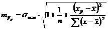 ,
,
where 
and the confidence interval of the forecast is built:
γ y x =y p Δ y p ; γ y x min=y p -Δ y p ; γ y x max=y p +Δ y p
where Δ y x =t table ·m y x .
Solution example
Task number 1. For seven territories of the Ural region For 199X, the values of two signs are known.Table 1.
Required: 1. To characterize the dependence of y on x, calculate the parameters of the following functions:
a) linear;
b) power law (previously it is necessary to perform the procedure of linearization of variables by taking the logarithm of both parts);
c) demonstrative;
d) equilateral hyperbola (you also need to figure out how to pre-linearize this model).
2. Evaluate each model through the average approximation error A and Fisher's F-test.
Solution (Option #1)
To calculate the parameters a and b of the linear regression y=a+b·x (the calculation can be done using a calculator).solve the system of normal equations with respect to a and b:
Based on the initial data, we calculate ∑y, ∑x, ∑y x, ∑x², ∑y²:
| y | x | yx | x2 | y2 | y x | y-y x | A i | |
| l | 68,8 | 45,1 | 3102,88 | 2034,01 | 4733,44 | 61,3 | 7,5 | 10,9 |
| 2 | 61,2 | 59,0 | 3610,80 | 3481,00 | 3745,44 | 56,5 | 4,7 | 7,7 |
| 3 | 59,9 | 57,2 | 3426,28 | 3271,84 | 3588,01 | 57,1 | 2,8 | 4,7 |
| 4 | 56,7 | 61,8 | 3504,06 | 3819,24 | 3214,89 | 55,5 | 1,2 | 2,1 |
| 5 | 55,0 | 58,8 | 3234,00 | 3457,44 | 3025,00 | 56,5 | -1,5 | 2,7 |
| 6 | 54,3 | 47,2 | 2562,96 | 2227,84 | 2948,49 | 60,5 | -6,2 | 11,4 |
| 7 | 49,3 | 55,2 | 2721,36 | 3047,04 | 2430,49 | 57,8 | -8,5 | 17,2 |
| Total | 405,2 | 384,3 | 22162,34 | 21338,41 | 23685,76 | 405,2 | 0,0 | 56,7 |
| Wed value (Total/n) | 57,89 y | 54,90 x | 3166,05 x y | 3048,34 x² | 3383,68 y² | X | X | 8,1 |
| s | 5,74 | 5,86 | X | X | X | X | X | X |
| s2 | 32,92 | 34,34 | X | X | X | X | X | X |

a=y -b x = 57.89+0.35 54.9 ≈ 76.88
Regression equation: y= 76,88 - 0,35X. With an increase in the average daily wage by 1 rub. the share of spending on the purchase of food products is reduced by an average of 0.35% points.
Calculate the linear coefficient of pair correlation: ![]()
Communication is moderate, reverse.
Let's determine the coefficient of determination: r² xy =(-0.35)=0.127
The 12.7% variation in the result is explained by the variation in the x factor. Substituting the actual values into the regression equation X, we determine the theoretical (calculated) values of y x . Let us find the value of the average approximation error A :
On average, the calculated values deviate from the actual ones by 8.1%.
Let's calculate the F-criterion: 
The obtained value indicates the need to accept the hypothesis H 0 about the random nature of the revealed dependence and the statistical insignificance of the parameters of the equation and the indicator of closeness of connection.
1b. The construction of the power model y=a x b is preceded by the procedure of linearization of variables. In the example, linearization is done by taking the logarithm of both sides of the equation:
lg y=lg a + b lg x
Y=C+b Y
where Y=lg(y), X=lg(x), C=lg(a).
For calculations, we use the data in Table. 1.3.
Table 1.3
| Y | X | YX | Y2 | x2 | y x | y-y x | (y-yx)² | A i | |
| 1 | 1,8376 | 1,6542 | 3,0398 | 3,3768 | 2,7364 | 61,0 | 7,8 | 60,8 | 11,3 |
| 2 | 1,7868 | 1,7709 | 3,1642 | 3,1927 | 3,1361 | 56,3 | 4,9 | 24,0 | 8,0 |
| 3 | 1,7774 | 1,7574 | 3,1236 | 3,1592 | 3,0885 | 56,8 | 3,1 | 9,6 | 5,2 |
| 4 | 1,7536 | 1,7910 | 3,1407 | 3,0751 | 3,2077 | 55,5 | 1,2 | 1,4 | 2,1 |
| 5 | 1,7404 | 1,7694 | 3,0795 | 3,0290 | 3,1308 | 56,3 | -1,3 | 1,7 | 2,4 |
| 6 | 1,7348 | 1,6739 | 2,9039 | 3,0095 | 2,8019 | 60,2 | -5,9 | 34,8 | 10,9 |
| 7 | 1,6928 | 1,7419 | 2,9487 | 2,8656 | 3,0342 | 57,4 | -8,1 | 65,6 | 16,4 |
| Total | 12,3234 | 12,1587 | 21,4003 | 21,7078 | 21,1355 | 403,5 | 1,7 | 197,9 | 56,3 |
| Mean | 1,7605 | 1,7370 | 3,0572 | 3,1011 | 3,0194 | X | X | 28,27 | 8,0 |
| σ | 0,0425 | 0,0484 | X | X | X | X | X | X | X |
| σ2 | 0,0018 | 0,0023 | X | X | X | X | X | X | X |
Calculate C and b:
C=Y -b X = 1.7605+0.298 1.7370 = 2.278126
We get a linear equation: Y=2.278-0.298 X
After potentiating it, we get: y=10 2.278 x -0.298
Substituting in this equation the actual values X, we get the theoretical values of the result. Based on them, we calculate the indicators: the tightness of the connection - the correlation index p xy and the average approximation error A . 
The characteristics of the power model indicate that it describes the relationship somewhat better than the linear function.
1c. The construction of the equation of the exponential curve y \u003d a b x is preceded by the procedure for linearizing the variables when taking the logarithm of both parts of the equation:
lg y=lg a + x lg b
Y=C+B x
For calculations, we use the table data.
| Y | x | Yx | Y2 | x2 | y x | y-y x | (y-yx)² | A i | |
| 1 | 1,8376 | 45,1 | 82,8758 | 3,3768 | 2034,01 | 60,7 | 8,1 | 65,61 | 11,8 |
| 2 | 1,7868 | 59,0 | 105,4212 | 3,1927 | 3481,00 | 56,4 | 4,8 | 23,04 | 7,8 |
| 3 | 1,7774 | 57,2 | 101,6673 | 3,1592 | 3271,84 | 56,9 | 3,0 | 9,00 | 5,0 |
| 4 | 1,7536 | 61,8 | 108,3725 | 3,0751 | 3819,24 | 55,5 | 1,2 | 1,44 | 2,1 |
| 5 | 1,7404 | 58,8 | 102,3355 | 3,0290 | 3457,44 | 56,4 | -1,4 | 1,96 | 2,5 |
| 6 | 1,7348 | 47,2 | 81,8826 | 3,0095 | 2227,84 | 60,0 | -5,7 | 32,49 | 10,5 |
| 7 | 1,6928 | 55,2 | 93,4426 | 2,8656 | 3047,04 | 57,5 | -8,2 | 67,24 | 16,6 |
| Total | 12,3234 | 384,3 | 675,9974 | 21,7078 | 21338,41 | 403,4 | -1,8 | 200,78 | 56,3 |
| Wed zn. | 1,7605 | 54,9 | 96,5711 | 3,1011 | 3048,34 | X | X | 28,68 | 8,0 |
| σ | 0,0425 | 5,86 | X | X | X | X | X | X | X |
| σ2 | 0,0018 | 34,339 | X | X | X | X | X | X | X |
The values of the regression parameters A and AT amounted to:
A=Y -B x = 1.7605+0.0023 54.9 = 1.887
A linear equation is obtained: Y=1.887-0.0023x. We potentiate the resulting equation and write it in the usual form:
y x =10 1.887 10 -0.0023x = 77.1 0.9947 x
We estimate the tightness of the relationship through the correlation index p xy: 
