Linear Equations with Two Variables
The student has 200 rubles to have lunch at school. A cake costs 25 rubles, and a cup of coffee costs 10 rubles. How many cakes and cups of coffee can you buy for 200 rubles?
Denote the number of cakes through x, and the number of cups of coffee through y. Then the cost of cakes will be denoted by the expression 25 x, and the cost of cups of coffee in 10 y .
25x- price x cakes
10y- price y cups of coffee
The total amount should be 200 rubles. Then we get an equation with two variables x and y
25x+ 10y= 200
How many roots does this equation have?
It all depends on the appetite of the student. If he buys 6 cakes and 5 cups of coffee, then the roots of the equation will be the numbers 6 and 5.
The pair of values 6 and 5 are said to be the roots of Equation 25 x+ 10y= 200 . Written as (6; 5) , with the first number being the value of the variable x, and the second - the value of the variable y .
6 and 5 are not the only roots that reverse Equation 25 x+ 10y= 200 to identity. If desired, for the same 200 rubles, a student can buy 4 cakes and 10 cups of coffee:

In this case, the roots of equation 25 x+ 10y= 200 is the pair of values (4; 10) .
Moreover, a student may not buy coffee at all, but buy cakes for all 200 rubles. Then the roots of equation 25 x+ 10y= 200 will be the values 8 and 0

Or vice versa, do not buy cakes, but buy coffee for all 200 rubles. Then the roots of equation 25 x+ 10y= 200 will be the values 0 and 20

Let's try to list all possible roots of equation 25 x+ 10y= 200 . Let us agree that the values x and y belong to the set of integers. And let these values be greater than or equal to zero:
x∈Z, y∈ Z;
x ≥ 0, y ≥ 0
So it will be convenient for the student himself. Cakes are more convenient to buy whole than, for example, several whole cakes and half a cake. Coffee is also more convenient to take in whole cups than, for example, several whole cups and half a cup.
Note that for odd x it is impossible to achieve equality under any y. Then the values x there will be the following numbers 0, 2, 4, 6, 8. And knowing x can be easily determined y

Thus, we got the following pairs of values (0; 20), (2; 15), (4; 10), (6; 5), (8; 0). These pairs are solutions or roots of Equation 25 x+ 10y= 200. They turn this equation into an identity.
Type equation ax + by = c called linear equation with two variables. A solution or roots of this equation is a pair of values ( x; y), which turns it into an identity.
Note also that if a linear equation with two variables is written as ax + b y = c , then they say that it is written in canonical(normal) form.
Some linear equations in two variables can be reduced to canonical form.
For example, the equation 2(16x+ 3y- 4) = 2(12 + 8x − y) can be brought to mind ax + by = c. Let's open the brackets in both parts of this equation, we get 32x + 6y − 8 = 24 + 16x − 2y . The terms containing unknowns are grouped on the left side of the equation, and the terms free of unknowns are grouped on the right. Then we get 32x - 16x+ 6y+ 2y = 24 + 8 . We bring similar terms in both parts, we get equation 16 x+ 8y= 32. This equation is reduced to the form ax + by = c and is canonical.
Equation 25 considered earlier x+ 10y= 200 is also a two-variable linear equation in canonical form. In this equation, the parameters a , b and c are equal to the values 25, 10 and 200, respectively.
Actually the equation ax + by = c has an infinite number of solutions. Solving the Equation 25x+ 10y= 200, we looked for its roots only on the set of integers. As a result, we obtained several pairs of values that turned this equation into an identity. But on the set of rational numbers equation 25 x+ 10y= 200 will have an infinite number of solutions.
To get new pairs of values, you need to take an arbitrary value for x, then express y. For example, let's take a variable x value 7. Then we get an equation with one variable 25×7 + 10y= 200 in which to express y

Let x= 15 . Then the equation 25x+ 10y= 200 becomes 25 × 15 + 10y= 200. From here we find that y = −17,5

Let x= −3 . Then the equation 25x+ 10y= 200 becomes 25 × (−3) + 10y= 200. From here we find that y = −27,5

System of two linear equations with two variables
For the equation ax + by = c you can take any number of times arbitrary values for x and find values for y. Taken separately, such an equation will have an infinite number of solutions.
But it also happens that the variables x and y connected not by one, but by two equations. In this case, they form the so-called system of linear equations with two variables. Such a system of equations can have one pair of values (or in other words: “one solution”).
It may also happen that the system has no solutions at all. A system of linear equations can have an infinite number of solutions in rare and exceptional cases.
Two linear equations form a system when the values x and y are included in each of these equations.
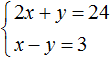
Let's go back to the very first equation 25 x+ 10y= 200 . One of the pairs of values for this equation was the pair (6; 5) . This is the case when 200 rubles could buy 6 cakes and 5 cups of coffee.
We compose the problem so that the pair (6; 5) becomes the only solution for equation 25 x+ 10y= 200 . To do this, we compose another equation that would connect the same x cakes and y cups of coffee.
Let's put the text of the task as follows:
“A schoolboy bought several cakes and several cups of coffee for 200 rubles. A cake costs 25 rubles, and a cup of coffee costs 10 rubles. How many cakes and cups of coffee did the student buy if it is known that the number of cakes is one more than the number of cups of coffee?
We already have the first equation. This is Equation 25 x+ 10y= 200 . Now let's write an equation for the condition "the number of cakes is one unit more than the number of cups of coffee" .
The number of cakes is x, and the number of cups of coffee is y. You can write this phrase using the equation x − y= 1. This equation would mean that the difference between cakes and coffee is 1.
x=y+ 1 . This equation means that the number of cakes is one more than the number of cups of coffee. Therefore, to obtain equality, one is added to the number of cups of coffee. This can be easily understood if we use the weight model that we considered when studying the simplest problems:

Got two equations: 25 x+ 10y= 200 and x=y+ 1. Since the values x and y, namely 6 and 5 are included in each of these equations, then together they form a system. Let's write down this system. If the equations form a system, then they are framed by the sign of the system. The system sign is a curly brace:

Let's solve this system. This will allow us to see how we arrive at the values 6 and 5. There are many methods for solving such systems. Consider the most popular of them.
Substitution Method
The name of this method speaks for itself. Its essence is to substitute one equation into another, having previously expressed one of the variables.
In our system, nothing needs to be expressed. In the second equation x = y+ 1 variable x already expressed. This variable is equal to the expression y+ 1 . Then you can substitute this expression in the first equation instead of the variable x

After substituting the expression y+ 1 into the first equation instead x, we get the equation 25(y+ 1) + 10y= 200 . This is a linear equation with one variable. This equation is quite easy to solve:

We found the value of the variable y. Now we substitute this value into one of the equations and find the value x. For this, it is convenient to use the second equation x = y+ 1 . Let's put the value into it y
So the pair (6; 5) is a solution to the system of equations, as we intended. We check and make sure that the pair (6; 5) satisfies the system:

Example 2

Substitute the first equation x= 2 + y into the second equation 3 x - 2y= 9 . In the first equation, the variable x is equal to the expression 2 + y. We substitute this expression into the second equation instead of x

Now let's find the value x. To do this, substitute the value y into the first equation x= 2 + y
So the solution of the system is the pair value (5; 3)
Example 3. Solve the following system of equations using the substitution method:

Here, unlike the previous examples, one of the variables is not explicitly expressed.
To substitute one equation into another, you first need .
It is desirable to express the variable that has a coefficient of one. The coefficient unit has a variable x, which is contained in the first equation x+ 2y= 11 . Let's express this variable.
After a variable expression x, our system will look like this:

Now we substitute the first equation into the second and find the value y

Substitute y x

So the solution of the system is a pair of values (3; 4)
Of course, you can also express a variable y. The roots will not change. But if you express y, the result is not a very simple equation, the solution of which will take more time. It will look like this:

We see that in this example to express x much more convenient than expressing y .
Example 4. Solve the following system of equations using the substitution method:

Express in the first equation x. Then the system will take the form:

y

Substitute y into the first equation and find x. You can use the original equation 7 x+ 9y= 8 , or use the equation in which the variable is expressed x. We will use this equation, since it is convenient:
![]()
So the solution of the system is the pair of values (5; −3)
Addition method
The addition method is to add term by term the equations included in the system. This addition results in a new one-variable equation. And it's pretty easy to solve this equation.
Let's solve the following system of equations:
Add the left side of the first equation to the left side of the second equation. And the right side of the first equation with the right side of the second equation. We get the following equality:
Here are similar terms:

As a result, we obtained the simplest equation 3 x= 27 whose root is 9. Knowing the value x you can find the value y. Substitute the value x into the second equation x − y= 3 . We get 9 − y= 3 . From here y= 6 .
So the solution of the system is a pair of values (9; 6)
Example 2

Add the left side of the first equation to the left side of the second equation. And the right side of the first equation with the right side of the second equation. In the resulting equality, we present like terms:

As a result, we got the simplest equation 5 x= 20, the root of which is 4. Knowing the value x you can find the value y. Substitute the value x into the first equation 2 x+y= 11 . Let's get 8 + y= 11 . From here y= 3 .
So the solution of the system is the pair of values (4;3)
The addition process is not described in detail. It has to be done in the mind. When adding, both equations must be reduced to canonical form. That is, to the mind ac+by=c .
From the considered examples, it can be seen that the main goal of adding equations is to get rid of one of the variables. But it is not always possible to immediately solve the system of equations by the addition method. Most often, the system is preliminarily brought to a form in which it is possible to add the equations included in this system.
For example, the system  can be solved directly by the addition method. When adding both equations, the terms y and −y vanish because their sum is zero. As a result, the simplest equation is formed 11 x= 22 , whose root is 2. Then it will be possible to determine y equal to 5.
And the system of equations  the addition method cannot be solved immediately, since this will not lead to the disappearance of one of the variables. Addition will result in Equation 8 x+ y= 28 , which has an infinite number of solutions.
If both parts of the equation are multiplied or divided by the same number that is not equal to zero, then an equation equivalent to the given one will be obtained. This rule is also valid for a system of linear equations with two variables. One of the equations (or both equations) can be multiplied by some number. The result is an equivalent system, the roots of which will coincide with the previous one.
Let's return to the very first system, which described how many cakes and cups of coffee the student bought. The solution of this system was a pair of values (6; 5) .
We multiply both equations included in this system by some numbers. Let's say we multiply the first equation by 2 and the second by 3
The result is a system 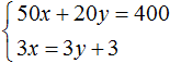
The solution to this system is still the pair of values (6; 5)
This means that the equations included in the system can be reduced to a form suitable for applying the addition method.
Back to the system , which we could not solve by the addition method.
Multiply the first equation by 6 and the second by −2

Then we get the following system:

We add the equations included in this system. Addition of components 12 x and -12 x will result in 0, addition 18 y and 4 y will give 22 y, and adding 108 and −20 gives 88. Then you get the equation 22 y= 88 , hence y = 4 .
If at first it is difficult to add equations in your mind, then you can write down how the left side of the first equation is added to the left side of the second equation, and the right side of the first equation to the right side of the second equation:

Knowing that the value of the variable y is 4, you can find the value x. Substitute y into one of the equations, for example into the first equation 2 x+ 3y= 18 . Then we get an equation with one variable 2 x+ 12 = 18 . We transfer 12 to the right side, changing the sign, we get 2 x= 6 , hence x = 3 .
Example 4. Solve the following system of equations using the addition method:

Multiply the second equation by −1. Then the system will take the following form:

Let's add both equations. Addition of components x and −x will result in 0, addition 5 y and 3 y will give 8 y, and adding 7 and 1 gives 8. The result is equation 8 y= 8 , whose root is 1. Knowing that the value y is 1, you can find the value x .
Substitute y into the first equation, we get x+ 5 = 7 , hence x= 2
Example 5. Solve the following system of equations using the addition method:

It is desirable that the terms containing the same variables are located one under the other. Therefore, in the second equation, the terms 5 y and −2 x change places. As a result, the system will take the form:

Multiply the second equation by 3. Then the system will take the form:

Now let's add both equations. As a result of addition, we get equation 8 y= 16 , whose root is 2.
Substitute y into the first equation, we get 6 x− 14 = 40 . We transfer the term −14 to the right side, changing the sign, we get 6 x= 54 . From here x= 9.
Example 6. Solve the following system of equations using the addition method:

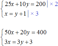
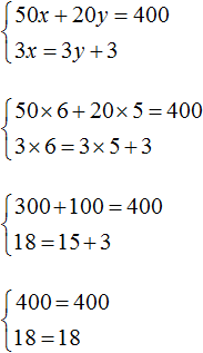
Let's get rid of fractions. Multiply the first equation by 36 and the second by 12
In the resulting system  the first equation can be multiplied by −5 and the second by 8

Let's add the equations in the resulting system. Then we get the simplest equation −13 y= −156 . From here y= 12 . Substitute y into the first equation and find x

Example 7. Solve the following system of equations using the addition method:

We bring both equations to normal form. Here it is convenient to apply the rule of proportion in both equations. If in the first equation the right side is represented as , and the right side of the second equation as , then the system will take the form:

We have a proportion. We multiply its extreme and middle terms. Then the system will take the form:

We multiply the first equation by −3, and open the brackets in the second:

Now let's add both equations. As a result of adding these equations, we get an equality, in both parts of which there will be zero:

It turns out that the system has an infinite number of solutions.
But we cannot simply take arbitrary values from the sky for x and y. We can specify one of the values, and the other will be determined depending on the value we specify. For example, let x= 2 . Substitute this value into the system:

As a result of solving one of the equations, the value for y, which will satisfy both equations:

The resulting pair of values (2; −2) will satisfy the system:
Let's find another pair of values. Let x= 4. Substitute this value into the system:

It can be determined by eye that y equals zero. Then we get a pair of values (4; 0), which satisfies our system:

Example 8. Solve the following system of equations using the addition method:

Multiply the first equation by 6 and the second by 12

Let's rewrite what's left:


Multiply the first equation by −1. Then the system will take the form:

Now let's add both equations. As a result of addition, equation 6 is formed b= 48 , whose root is 8. Substitute b into the first equation and find a

System of linear equations with three variables
A linear equation with three variables includes three variables with coefficients, as well as an intercept. In canonical form, it can be written as follows:
ax + by + cz = d
This equation has an infinite number of solutions. By giving two variables different values, a third value can be found. The solution in this case is the triple of values ( x; y; z) which turns the equation into an identity.
If variables x, y, z are interconnected by three equations, then a system of three linear equations with three variables is formed. To solve such a system, you can apply the same methods that apply to linear equations with two variables: the substitution method and the addition method.
Example 1. Solve the following system of equations using the substitution method:

We express in the third equation x. Then the system will take the form:

Now let's do the substitution. Variable x is equal to the expression 3 − 2y − 2z . Substitute this expression into the first and second equations:

Let's open the brackets in both equations and give like terms:

We have arrived at a system of linear equations with two variables. In this case, it is convenient to apply the addition method. As a result, the variable y will disappear and we can find the value of the variable z
![]()
Now let's find the value y. For this, it is convenient to use the equation − y+ z= 4. Substitute the value z

Now let's find the value x. For this, it is convenient to use the equation x= 3 − 2y − 2z . Substitute the values into it y and z

Thus, the triple of values (3; −2; 2) is the solution to our system. By checking, we make sure that these values satisfy the system:

Example 2. Solve the system by addition method

Let's add the first equation with the second multiplied by −2.
If the second equation is multiplied by −2, then it will take the form −6x+ 6y- 4z = −4 . Now add it to the first equation:

We see that as a result of elementary transformations, the value of the variable was determined x. It is equal to one.
Let's go back to the main system. Let's add the second equation with the third multiplied by −1. If the third equation is multiplied by −1, then it will take the form −4x + 5y − 2z = −1 . Now add it to the second equation:

Got the equation x - 2y= −1 . Substitute the value into it x which we found earlier. Then we can determine the value y

We now know the values x and y. This allows you to determine the value z. We use one of the equations included in the system:

Thus, the triple of values (1; 1; 1) is the solution to our system. By checking, we make sure that these values satisfy the system:

Tasks for compiling systems of linear equations
The task of compiling systems of equations is solved by introducing several variables. Next, equations are compiled based on the conditions of the problem. From the compiled equations, they form a system and solve it. Having solved the system, it is necessary to check whether its solution satisfies the conditions of the problem.
Task 1. A Volga car left the city for the collective farm. She returned back along another road, which was 5 km shorter than the first. In total, the car drove 35 km both ways. How many kilometers is each road long?
Solution
Let x- length of the first road, y- the length of the second. If the car drove 35 km both ways, then the first equation can be written as x+ y= 35. This equation describes the sum of the lengths of both roads.
It is said that the car was returning back along the road, which was shorter than the first one by 5 km. Then the second equation can be written as x− y= 5. This equation shows that the difference between the lengths of the roads is 5 km.
Or the second equation can be written as x= y+ 5 . We will use this equation.
Since the variables x and y in both equations denote the same number, then we can form a system from them:
Let's solve this system using one of the previously studied methods. In this case, it is convenient to use the substitution method, since in the second equation the variable x already expressed.
Substitute the second equation into the first and find y
Substitute the found value y into the second equation x= y+ 5 and find x
The length of the first road was denoted by the variable x. Now we have found its meaning. Variable x is 20. So the length of the first road is 20 km.
And the length of the second road was indicated by y. The value of this variable is 15. So the length of the second road is 15 km.
Let's do a check. First, let's make sure that the system is solved correctly:

Now let's check whether the solution (20; 15) satisfies the conditions of the problem.
It was said that in total the car drove 35 km both ways. We add up the lengths of both roads and make sure that the solution (20; 15) satisfies this condition: 20 km + 15 km = 35 km
Next condition: the car returned back along another road, which was 5 km shorter than the first . We see that the solution (20; 15) also satisfies this condition, since 15 km is shorter than 20 km by 5 km: 20 km − 15 km = 5 km
When compiling a system, it is important that the variables denote the same numbers in all equations included in this system.
So our system contains two equations. These equations in turn contain the variables x and y, which denote the same numbers in both equations, namely the lengths of roads equal to 20 km and 15 km.
Task 2. Oak and pine sleepers were loaded onto the platform, a total of 300 sleepers. It is known that all oak sleepers weighed 1 ton less than all pine sleepers. Determine how many oak and pine sleepers there were separately, if each oak sleeper weighed 46 kg, and each pine sleeper 28 kg.
Solution
Let x oak and y pine sleepers were loaded onto the platform. If there were 300 sleepers in total, then the first equation can be written as x+y = 300 .
All oak sleepers weighed 46 x kg, and pine weighed 28 y kg. Since oak sleepers weighed 1 ton less than pine sleepers, the second equation can be written as 28y- 46x= 1000 . This equation shows that the mass difference between oak and pine sleepers is 1000 kg.
Tons have been converted to kilograms because the mass of oak and pine sleepers is measured in kilograms.
As a result, we obtain two equations that form the system

Let's solve this system. Express in the first equation x. Then the system will take the form:

Substitute the first equation into the second and find y

Substitute y into the equation x= 300 − y and find out what x

This means that 100 oak and 200 pine sleepers were loaded onto the platform.
Let's check whether the solution (100; 200) satisfies the conditions of the problem. First, let's make sure that the system is solved correctly:

It was said that there were 300 sleepers in total. We add up the number of oak and pine sleepers and make sure that the solution (100; 200) satisfies this condition: 100 + 200 = 300.
Next condition: all oak sleepers weighed 1 ton less than all pine . We see that the solution (100; 200) also satisfies this condition, since 46 × 100 kg of oak sleepers are lighter than 28 × 200 kg of pine sleepers: 5600 kg − 4600 kg = 1000 kg.
Task 3. We took three pieces of an alloy of copper and nickel in ratios of 2: 1, 3: 1 and 5: 1 by weight. Of these, a piece weighing 12 kg was fused with a ratio of copper and nickel content of 4: 1. Find the mass of each original piece if the mass of the first of them is twice the mass of the second.
Let us first consider the case when the number of equations is equal to the number of variables, i.e. m = n. Then the matrix of the system is square, and its determinant is called the determinant of the system.
Inverse matrix method
Consider in general terms the system of equations AX = B with a non-singular square matrix A. In this case, there is an inverse matrix A -1 . Let's multiply both sides by A -1 on the left. We get A -1 AX \u003d A -1 B. From here EX \u003d A -1 B and
The last equality is a matrix formula for finding solutions to such systems of equations. The use of this formula is called the inverse matrix method
For example, let's use this method to solve the following system:

 ;
;


At the end of the solution of the system, a check can be made by substituting the found values into the equations of the system. In this case, they must turn into true equalities.
For this example, let's check:

Method for solving systems of linear equations with a square matrix using Cramer's formulas
Let n=2:

If both parts of the first equation are multiplied by a 22, and both parts of the second by (-a 12), and then the resulting equations are added, then we will exclude the variable x 2 from the system. Similarly, you can eliminate the variable x 1 (by multiplying both sides of the first equation by (-a 21) and both sides of the second by a 11). As a result, we get the system:

The expression in brackets is the determinant of the system

Denote
Then the system will take the form:

It follows from the resulting system that if the determinant of the system is 0, then the system will be consistent and definite. Its unique solution can be calculated by the formulas:

If = 0, a 1 0 and/or 2 0, then the equations of the system will take the form 0*х 1 = 2 and/or 0*х 1 = 2. In this case, the system will be inconsistent.
In the case when = 1 = 2 = 0, the system will be consistent and indefinite (it will have an infinite number of solutions), as it will take the form:

Cramer's theorem(we omit the proof). If the determinant of the matrix of the system n of equations is not equal to zero, then the system has a unique solution, determined by the formulas:
 ,
,
where j is the determinant of the matrix obtained from the matrix A by replacing the j-th column with a column of free members.
The above formulas are called Cramer's formulas.
As an example, let's use this method to solve a system that was previously solved using the inverse matrix method:


Disadvantages of the considered methods:
1) significant complexity (calculation of determinants and finding the inverse matrix);
2) limited scope (for systems with a square matrix).
Real economic situations are often modeled by systems in which the number of equations and variables is quite significant, and there are more equations than variables. Therefore, the following method is more common in practice.
Gauss method (method of successive elimination of variables)
This method is used to solve a system of m linear equations with n variables in a general way. Its essence lies in applying a system of equivalent transformations to the expanded matrix, with the help of which the system of equations is transformed to the form when its solutions become easy to find (if any).
This is such a view in which the upper left part of the system matrix will be a stepped matrix. This is achieved using the same techniques that were used to obtain a stepped matrix in order to determine the rank. In this case, elementary transformations are applied to the expanded matrix, which will allow one to obtain an equivalent system of equations. After that, the augmented matrix will take the form:

Obtaining such a matrix is called in a straight line Gauss method.
Finding the values of variables from the corresponding system of equations is called backwards Gauss method. Let's consider it.
Note that the last (m – r) equations will take the form:
If at least one of the numbers  is not equal to zero, then the corresponding equality will be false, and the whole system will be inconsistent.
Therefore, for any joint system  . In this case, the last (m – r) equations for any values of the variables will be identities 0 = 0, and they can be ignored when solving the system (just discard the corresponding rows).
After that, the system will look like:

Consider first the case when r=n. Then the system will take the form:

From the last equation of the system one can uniquely find x r .
Knowing x r , one can uniquely express x r -1 from it. Then from the previous equation, knowing x r and x r -1 , we can express x r -2 and so on. up to x 1 .
So, in this case, the system will be collaborative and definite.


Now consider the case when r
From this equation, we can express the basic variable x r in terms of non-basic ones:

The penultimate equation will look like:
Substituting the resulting expression instead of x r, it will be possible to express the basic variable x r -1 through non-basic ones. Etc. to variable x 1 . To obtain a solution to the system, you can equate non-basic variables to arbitrary values and then calculate the basic variables using the obtained formulas. Thus, in this case, the system will be consistent and indeterminate (have an infinite number of solutions).
For example, let's solve the system of equations:


The set of basic variables will be called basis systems. The set of columns of coefficients for them will also be called basis(basic columns), or basic minor system matrices. That solution of the system, in which all non-basic variables are equal to zero, will be called basic solution.
In the previous example, the basic solution will be (4/5; -17/5; 0; 0) (variables x 3 and x 4 (c 1 and c 2) are set to zero, and the basic variables x 1 and x 2 are calculated through them) . To give an example of a non-basic solution, it is necessary to equate x 3 and x 4 (c 1 and c 2) to arbitrary numbers that are not equal to zero at the same time, and calculate the rest of the variables through them. For example, with c 1 = 1 and c 2 = 0, we get a non-basic solution - (4/5; -12/5; 1; 0). By substitution, it is easy to verify that both solutions are correct.
Obviously, in an indefinite system of non-basic solutions, there can be an infinite number of solutions. How many basic solutions can there be? Each row of the transformed matrix must correspond to one basic variable. In total, there are n variables in the problem, and r basic rows. Therefore, the number of possible sets of basic variables cannot exceed the number of combinations from n to 2 . It may be less than  , because it is not always possible to transform the system to such a form that this particular set of variables is the basis.
What kind is this? This is such a form when the matrix formed from the columns of the coefficients for these variables will be stepwise and, in this case, will consist of rrows. Those. the rank of the matrix of coefficients for these variables must be equal to r. It cannot be larger, since the number of columns is equal to r. If it turns out to be less than r, then this indicates a linear dependence of the columns with variables. Such columns cannot form a basis.
Let us consider what other basic solutions can be found in the above example. To do this, consider all possible combinations of four variables with two basic ones. Such combinations will  , and one of them (x 1 and x 2) has already been considered.
Let's take variables x 1 and x 3 . Find the rank of the matrix of coefficients for them:

Since it is equal to two, they can be basic. We equate the non-basic variables x 2 and x 4 to zero: x 2 \u003d x 4 \u003d 0. Then from the formula x 1 \u003d 4/5 - (1/5) * x 4 it follows that x 1 \u003d 4/5, and from the formula x 2 \u003d -17/5 + x 3 - - (7/5) * x 4 \u003d -17/5 + x 3 it follows that x 3 \u003d x 2 + 17/5 \u003d 17/5. Thus, we get the basic solution (4/5; 0; 17/5; 0).
Similarly, you can get basic solutions for the basic variables x 1 and x 4 - (9/7; 0; 0; -17/7); x 2 and x 4 - (0; -9; 0; 4); x 3 and x 4 - (0; 0; 9; 4).
The variables x 2 and x 3 in this example cannot be taken as basic ones, since the rank of the corresponding matrix is equal to one, i.e. less than two:
 .
.
Another approach is possible to determine whether or not it is possible to form a basis from some variables. When solving the example, as a result of transforming the system matrix to a stepped form, it took the form:

By choosing pairs of variables, it was possible to calculate the corresponding minors of this matrix. It is easy to see that for all pairs, except for x 2 and x 3 , they are not equal to zero, i.e. the columns are linearly independent. And only for columns with variables x 2 and x 3  , which indicates their linear dependence.
Let's consider one more example. Let's solve the system of equations


So, the equation corresponding to the third row of the last matrix is inconsistent - it led to the wrong equality 0 = -1, therefore, this system is inconsistent.
Jordan-Gauss method 3 is a development of the Gaussian method. Its essence is that the extended matrix of the system is transformed to the form when the coefficients of the variables form an identity matrix up to permutation of rows or columns 4 (where is the rank of the system matrix).
Let's solve the system using this method:

Consider the augmented matrix of the system:

In this matrix, we select the identity element. For example, the coefficient at x 2 in the third constraint is 5. Let's make sure that in the remaining rows in this column there are zeros, i.e. make the column single. In the process of transformations, we will call this columnpermissive(leading, key). The third constraint (the third string) will also be called permissive. Myself element, which stands at the intersection of the allowing row and column (here it is a unit), is also called permissive.
The first line now contains the coefficient (-1). To get zero in its place, multiply the third row by (-1) and subtract the result from the first row (i.e. just add the first row to the third).
The second line contains a coefficient of 2. To get zero in its place, multiply the third line by 2 and subtract the result from the first line.
The result of the transformations will look like:

This matrix clearly shows that one of the first two constraints can be deleted (the corresponding rows are proportional, i.e. these equations follow from each other). Let's cross out the second one:

So, there are two equations in the new system. A single column (second) is received, and the unit here is in the second row. Let's remember that the basic variable x 2 will correspond to the second equation of the new system.
Let's choose a basic variable for the first row. It can be any variable except x 3 (because at x 3 the first constraint has a zero coefficient, i.e. the set of variables x 2 and x 3 cannot be basic here). You can take the first or fourth variable.
Let's choose x 1. Then the resolving element will be 5, and both sides of the resolving equation will have to be divided by five in order to get one in the first column of the first row.
Let's make sure that the rest of the rows (i.e., the second row) have zeros in the first column. Since now the second line is not zero, but 3, it is necessary to subtract from the second line the elements of the converted first line, multiplied by 3:

One basic solution can be directly extracted from the resulting matrix by equating the non-basic variables to zero, and the basic variables to the free terms in the corresponding equations: (0.8; -3.4; 0; 0). You can also derive general formulas expressing basic variables through non-basic ones: x 1 \u003d 0.8 - 1.2 x 4; x 2 \u003d -3.4 + x 3 + 1.6x 4. These formulas describe the entire infinite set of solutions to the system (by equating x 3 and x 4 to arbitrary numbers, you can calculate x 1 and x 2).
Note that the essence of the transformations at each stage of the Jordan-Gauss method was as follows:
1) the permissive string was divided by the permissive element to get a unit in its place,
2) from all other rows, the transformed resolving power multiplied by the element that was in the given line in the resolving column was subtracted to get zero in place of this element.
Consider once again the transformed augmented matrix of the system:

It can be seen from this entry that the rank of the matrix of system A is r.
In the course of the above reasoning, we have established that the system is consistent if and only if  . This means that the augmented matrix of the system will look like:

Discarding zero rows, we get that the rank of the extended matrix of the system is also equal to r.
Kronecker-Capelli theorem. A system of linear equations is consistent if and only if the rank of the matrix of the system is equal to the rank of the extended matrix of this system.
Recall that the rank of a matrix is equal to the maximum number of its linearly independent rows. It follows from this that if the rank of the extended matrix is less than the number of equations, then the equations of the system are linearly dependent, and one or more of them can be excluded from the system (because they are a linear combination of the others). The system of equations will be linearly independent only if the rank of the extended matrix is equal to the number of equations.
Moreover, for compatible systems of linear equations, it can be argued that if the rank of the matrix is equal to the number of variables, then the system has a unique solution, and if it is less than the number of variables, then the system is indefinite and has infinitely many solutions.
1For example, suppose there are five rows in the matrix (the initial row order is 12345). We need to change the second line and the fifth. In order for the second line to take the place of the fifth, to “move” down, we sequentially change the adjacent lines three times: the second and third (13245), the second and fourth (13425) and the second and fifth (13452). Then, in order for the fifth row to take the place of the second in the original matrix, it is necessary to “shift” the fifth row up by only two consecutive changes: the fifth and fourth rows (13542) and the fifth and third (15342).
2Number of combinations from n to r  call the number of all different r-element subsets of an n-element set (different sets are those that have a different composition of elements, the selection order is not important). It is calculated by the formula:
  . Recall the meaning of the sign “!” (factorial):
  0!=1.)
3Since this method is more common than the Gauss method discussed earlier, and in essence is a combination of the forward and reverse Gauss method, it is also sometimes called the Gauss method, omitting the first part of the name.
4For example,  .
.
5If there were no units in the matrix of the system, then it would be possible, for example, to divide both parts of the first equation by two, and then the first coefficient would become unity; or the like.
Solve the system with two unknowns - this means finding all pairs of variable values that satisfy each of the given equations. Each such pair is called system solution.
Example:
The pair of values \(x=3\);\(y=-1\) is a solution to the first system, because by substituting these triples and minus ones into the system instead of \(x\) and \(y\), both equations become into valid equalities \(\begin(cases)3-2\cdot (-1)=5 \\3 \cdot 3+2 \cdot (-1)=7 \end(cases)\)
But \(x=1\); \(y=-2\) - is not a solution to the first system, because after substitution the second equation "does not converge" \(\begin(cases)1-2\cdot(-2)=5 \\3\cdot1+2 \cdot(-2)≠7 \end(cases)\)
Note that such pairs are often written shorter: instead of "\(x=3\); \(y=-1\)" they write like this: \((3;-1)\).
How to solve a system of linear equations?
There are three main ways to solve systems of linear equations:
- Substitution method.
-
\(\begin(cases)13x+9y=17\\12x-2y=26\end(cases)\)
In the second equation, each term is even, so we simplify the equation by dividing it by \(2\).
\(\begin(cases)13x+9y=17\\6x-y=13\end(cases)\)
This system can be solved in any of the ways, but it seems to me that the substitution method is the most convenient here. Let's express y from the second equation.
\(\begin(cases)13x+9y=17\\y=6x-13\end(cases)\)
Substitute \(6x-13\) for \(y\) in the first equation.
\(\begin(cases)13x+9(6x-13)=17\\y=6x-13\end(cases)\)
The first equation has become normal. We solve it.
Let's open the parentheses first.
\(\begin(cases)13x+54x-117=17\\y=6x-13\end(cases)\)
Let's move \(117\) to the right and give like terms.
\(\begin(cases)67x=134\\y=6x-13\end(cases)\)
Divide both sides of the first equation by \(67\).
\(\begin(cases)x=2\\y=6x-13\end(cases)\)
Hooray, we found \(x\)! Substitute its value into the second equation and find \(y\).
\(\begin(cases)x=2\\y=12-13\end(cases)\)\(\Leftrightarrow\)\(\begin(cases)x=2\\y=-1\end(cases )\)
Let's write down the answer.
\(\begin(cases)x-2y=5\\3x+2y=7 \end(cases)\)\(\Leftrightarrow\) \(\begin(cases)x=5+2y\\3x+2y= 7\end(cases)\)\(\Leftrightarrow\)
Substitute the resulting expression instead of this variable into another equation of the system.
\(\Leftrightarrow\) \(\begin(cases)x=5+2y\\3(5+2y)+2y=7\end(cases)\)\(\Leftrightarrow\)
We will analyze two types of solving systems of equations:
1. Solution of the system by the substitution method.
2. Solution of the system by term-by-term addition (subtraction) of the equations of the system.
In order to solve the system of equations substitution method you need to follow a simple algorithm:
1. We express. From any equation, we express one variable.
2. Substitute. We substitute in another equation instead of the expressed variable, the resulting value.
3. We solve the resulting equation with one variable. We find a solution to the system.
To solve system by term-by-term addition (subtraction) need:
1. Select a variable for which we will make the same coefficients.
2. We add or subtract the equations, as a result we get an equation with one variable.
3. We solve the resulting linear equation. We find a solution to the system.
The solution of the system is the intersection points of the graphs of the function.
Let us consider in detail the solution of systems using examples.
Example #1:
Let's solve by the substitution method
Solving the system of equations by the substitution method2x+5y=1 (1 equation)
x-10y=3 (2nd equation)
1. Express
It can be seen that in the second equation there is a variable x with a coefficient of 1, hence it turns out that it is easiest to express the variable x from the second equation.
x=3+10y
2. After expressing, we substitute 3 + 10y in the first equation instead of the variable x.
2(3+10y)+5y=1
3. We solve the resulting equation with one variable.
2(3+10y)+5y=1 (open brackets)
6+20y+5y=1
25y=1-6
25y=-5 |: (25)
y=-5:25
y=-0.2
The solution of the equation system is the intersection points of the graphs, therefore we need to find x and y, because the intersection point consists of x and y. Let's find x, in the first paragraph where we expressed we substitute y there.
x=3+10y
x=3+10*(-0.2)=1
It is customary to write points in the first place, we write the variable x, and in the second place the variable y.
Answer: (1; -0.2)
Example #2:
Let's solve by term-by-term addition (subtraction).
Solving a system of equations by the addition method3x-2y=1 (1 equation)
2x-3y=-10 (2nd equation)
1. Select a variable, let's say we select x. In the first equation, the variable x has a coefficient of 3, in the second - 2. We need to make the coefficients the same, for this we have the right to multiply the equations or divide by any number. We multiply the first equation by 2, and the second by 3 and get a total coefficient of 6.
3x-2y=1 |*2
6x-4y=2
2x-3y=-10 |*3
6x-9y=-30
2. From the first equation, subtract the second to get rid of the variable x. Solve the linear equation.
__6x-4y=2
5y=32 | :5
y=6.4
3. Find x. We substitute the found y in any of the equations, let's say in the first equation.
3x-2y=1
3x-2*6.4=1
3x-12.8=1
3x=1+12.8
3x=13.8 |:3
x=4.6
The point of intersection will be x=4.6; y=6.4
Answer: (4.6; 6.4)
Do you want to prepare for exams for free? Tutor online is free. No kidding.
More reliable than the graphical method discussed in the previous paragraph.
Substitution Method
We used this method in the 7th grade to solve systems of linear equations. The algorithm that was developed in the 7th grade is quite suitable for solving systems of any two equations (not necessarily linear) with two variables x and y (of course, the variables can be denoted by other letters, which does not matter). In fact, we used this algorithm in the previous paragraph, when the problem of a two-digit number led to a mathematical model, which is a system of equations. We solved this system of equations above by the substitution method (see example 1 from § 4).
Algorithm for using the substitution method when solving a system of two equations with two variables x, y.
1. Express y in terms of x from one equation of the system.
2. Substitute the resulting expression instead of y into another equation of the system.
3. Solve the resulting equation for x.
4. Substitute in turn each of the roots of the equation found at the third step instead of x into the expression y through x obtained at the first step.
5. Write down the answer in the form of pairs of values (x; y), which were found, respectively, in the third and fourth steps.

4) Substitute in turn each of the found values of y into the formula x \u003d 5 - Zy. If then ![]()
5) Pairs (2; 1) and solutions of a given system of equations.
Answer: (2; 1);
Algebraic addition method
This method, like the substitution method, is familiar to you from the 7th grade algebra course, where it was used to solve systems of linear equations. We recall the essence of the method in the following example.
Example 2 Solve a system of equations

We multiply all the terms of the first equation of the system by 3, and leave the second equation unchanged: 
Subtract the second equation of the system from its first equation:

As a result of algebraic addition of two equations of the original system, an equation was obtained that is simpler than the first and second equations of the given system. With this simpler equation, we have the right to replace any equation of a given system, for example, the second one. Then the given system of equations will be replaced by a simpler system:

This system can be solved by the substitution method. From the second equation we find Substituting this expression instead of y into the first equation of the system, we obtain

It remains to substitute the found values \u200b\u200bof x into the formula
If x = 2 then
Thus, we have found two solutions to the system: ![]()
Method for introducing new variables
You got acquainted with the method of introducing a new variable when solving rational equations with one variable in the 8th grade algebra course. The essence of this method for solving systems of equations is the same, but from a technical point of view there are some features that we will discuss in the following examples.
Example 3 Solve a system of equations

Let's introduce a new variable Then the first equation of the system can be rewritten in a simpler form: Let's solve this equation with respect to the variable t:

Both of these values satisfy the condition , and therefore are the roots of a rational equation with the variable t. But that means either from where we find that x = 2y, or
Thus, using the method of introducing a new variable, we managed, as it were, to “stratify” the first equation of the system, which is quite complex in appearance, into two simpler equations:
x = 2 y; y - 2x.
What's next? And then each of the two simple equations obtained must be considered in turn in a system with the equation x 2 - y 2 \u003d 3, which we have not yet remembered. In other words, the problem is reduced to solving two systems of equations:
![]()
It is necessary to find solutions for the first system, the second system, and include all the resulting pairs of values in the answer. Let's solve the first system of equations:
Let's use the substitution method, especially since everything is ready for it here: we substitute the expression 2y instead of x into the second equation of the system. Get

Since x \u003d 2y, we find x 1 \u003d 2, x 2 \u003d 2, respectively. Thus, two solutions to the given system are obtained: (2; 1) and (-2; -1). Let's solve the second system of equations:
Let's use the substitution method again: we substitute the expression 2x instead of y in the second equation of the system. Get

This equation has no roots, which means that the system of equations has no solutions. Thus, only the solutions of the first system should be included in the answer.
Answer: (2; 1); (-2;-1).
The method of introducing new variables in solving systems of two equations with two variables is used in two versions. First option: one new variable is introduced and used in only one equation of the system. This is exactly what happened in example 3. The second option: two new variables are introduced and used simultaneously in both equations of the system. This will be the case in example 4.
Example 4 Solve a system of equations

Let's introduce two new variables:
![]()
We learn that then
![]()
This will allow us to rewrite the given system in a much simpler form, but with respect to the new variables a and b:

Since a \u003d 1, then from the equation a + 6 \u003d 2 we find: 1 + 6 \u003d 2; 6=1. Thus, for the variables a and b, we got one solution:
Returning to the variables x and y, we obtain the system of equations

We apply the algebraic addition method to solve this system:

Since then from the equation 2x + y = 3 we find:
Thus, for the variables x and y, we got one solution:
Let us conclude this section with a brief but rather serious theoretical discussion. You have already gained some experience in solving various equations: linear, square, rational, irrational. You know that the main idea of solving an equation is to gradually move from one equation to another, simpler but equivalent to the given one. In the previous section, we introduced the notion of equivalence for equations with two variables. This concept is also used for systems of equations.
Definition.
Two systems of equations with variables x and y are said to be equivalent if they have the same solutions or if both systems have no solutions.
All three methods (substitution, algebraic addition, and introduction of new variables) that we have discussed in this section are absolutely correct from the point of view of equivalence. In other words, using these methods, we replace one system of equations with another, simpler, but equivalent to the original system.
Graphical method for solving systems of equations
We have already learned how to solve systems of equations in such common and reliable ways as the method of substitution, algebraic addition and the introduction of new variables. And now let's remember the method that you already studied in the previous lesson. That is, let's repeat what you know about the graphical solution method.
The method of solving systems of equations graphically is the construction of a graph for each of the specific equations that are included in this system and are in the same coordinate plane, and also where it is required to find the intersection of the points of these graphs. To solve this system of equations are the coordinates of this point (x; y).
It should be remembered that for a graphical system of equations it is common to have either one single correct solution, or an infinite number of solutions, or not to have solutions at all.
Now let's take a closer look at each of these solutions. And so, the system of equations can have a unique solution if the lines, which are the graphs of the equations of the system, intersect. If these lines are parallel, then such a system of equations has absolutely no solutions. In the case of the coincidence of the direct graphs of the equations of the system, then such a system allows you to find many solutions.
Well, now let's take a look at the algorithm for solving a system of two equations with 2 unknowns using a graphical method:
First, at first we build a graph of the 1st equation;
The second step will be to plot a graph that relates to the second equation;
Thirdly, we need to find the intersection points of the graphs.
And as a result, we get the coordinates of each intersection point, which will be the solution to the system of equations.
Let's look at this method in more detail with an example. We are given a system of equations to be solved:

Solving Equations
1. First, we will build a graph of this equation: x2+y2=9.
But it should be noted that this graph of equations will be a circle centered at the origin, and its radius will be equal to three.
2. Our next step will be to plot an equation such as: y = x - 3.
In this case, we must build a line and find the points (0;−3) and (3;0).

3. Let's see what we got. We see that the line intersects the circle at two of its points A and B.
Now we are looking for the coordinates of these points. We see that the coordinates (3;0) correspond to point A, and the coordinates (0;−3) correspond to point B.
And what do we get as a result?
The numbers (3;0) and (0;−3) obtained at the intersection of a straight line with a circle are precisely the solutions of both equations of the system. And from this it follows that these numbers are also solutions of this system of equations.
That is, the answer of this solution is the numbers: (3;0) and (0;−3).
