Page 1

The oscillatory process in the low-voltage circuit stops already during the first period of high-frequency oscillations, since in the second half of the period of these oscillations, the direction of the current becomes opposite to the current in the power circuit. To increase the brightness of the spark in the generator, it is possible to further increase the capacitance.

Oscillatory processes cover a wide range of phenomena, which are characterized by the repetition of their characteristics through certain intervals time.

An oscillatory process occurs in a system when, along with a force that brings it out of equilibrium, there is also a restoring (returning) force. What will happen if the restoring force acts on the system with some constant delay. Moreover, if such instability associated with the effects of delay is harmful to the ship's stabilizing mechanisms, then it is useful in the development of electronic generators.

The oscillatory processes that determine the magnitude of the dynamic loads on the rods essentially determine the shape of the dynamo-grams recorded near the polished rod.

The oscillatory process in the circuit occurs under non-zero initial conditions. The initial current in the inductance x is determined from the following considerations. Switch B breaks the circuit when the current tB - i0 - ic passes through zero.

Oscillatory processes can also occur in electrical machines and other electrical installations with significant inductance and rotating masses, when switching on, off and on. abrupt changes operating mode. Under certain conditions, not damped, but swinging oscillations appear. Such fluctuations can lead to serious violations operation of electrical installations and even cause accidents. Therefore, when developing control systems for electrical machines and other installations, in some cases it is necessary to apply special measures for the fastest attenuation of oscillatory processes (introduce resistances into their circuits, etc.).

Oscillatory processes and oscillatory boundaries of stability of various nonlinear systems can often be determined by harmonic linearization, the concept of which was given above. There are other methods as well. The most effective here are the numerical-graphical methods for constructing transient processes, as well as, especially, the methods of electrical simulation on mathematical machines of continuous and discrete action.

Oscillatory processes and oscillatory boundaries of stability of various nonlinear systems can often be determined by the method of harmonic linearization, the concept of which was given above.

Oscillatory processes are widespread in nature and technology. The swing of the pendulum of a clock, waves on water, alternating electric current, light, sound are examples of the oscillations of various physical quantities. When the pendulum moves, the coordinate of its center of gravity fluctuates. When alternating current voltage and current fluctuate in the circuit. These two processes are qualitatively completely different in their physical nature. However, the quantitative regularities of these processes have a lot in common.

Oscillatory processes in the rods are caused not only by the operation of surface equipment, but also by the movement of the plunger. Here, synchronous oscillations are more desirable, since in this case they do not cause overload.

Oscillatory processes are widespread in nature and technology. The swing of a pendulum of a clock, waves on water, alternating electric current, light, sound are examples of oscillations of various physical quantities. When the pendulum moves, the coordinate of its center of gravity fluctuates. In the case of alternating current, the voltage and current in the circuit fluctuate. These two processes are qualitatively completely different in their physical nature. However, the quantitative regularities of these processes have a lot in common.

Free vibrations in the circuit.

The AC circuits considered in the previous sections suggest that a pair of elements - a capacitor and an inductor form a kind of oscillatory system. Now we will show that this is indeed the case, in a circuit consisting only of these elements (Fig. 669), even free vibrations are possible, that is, without external source EMF.

rice. 669
Therefore, a circuit (or part of another circuit) consisting of a capacitor and an inductor is called oscillatory circuit.
Let the capacitor be charged to a charge qo and then an inductor connected to it. Such a procedure can be easily carried out using the circuit, the scheme of which is shown in Fig. 670: first the key is closed in position 1 , while the capacitor is charged to a voltage equal to source emf, after which the key is thrown into positions 2 , after which the discharge of the capacitor through the coil begins.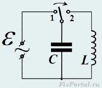

rice. 670
To determine the dependence of the charge of the capacitor on time q(t) apply Ohm's law, according to which the voltage across the capacitor U C = q/C equals EMF self-induction, arising in the coil

here, "prime" means derivative with respect to time.
Thus, the equation turns out to be valid

This equation contains two unknown functions - the dependence on the charge time q(t) and current I(t), so it cannot be solved. However, the current strength is a derivative of the charge of the capacitor q / (t) = I(t), so the derivative of the current strength is the second derivative of the charge

Taking into account this relation, we rewrite equation (1) in the form

Surprisingly, this equation completely coincides with the well-studied equation of harmonic oscillations (the second derivative of the unknown function is proportional to this function itself with a negative coefficient of proportionality x // = −ω o 2 x)! Therefore, the solution to this equation will be the harmonic function

with circular frequency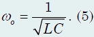

This formula defines natural frequency of the oscillatory circuit. Accordingly, the oscillation period of the capacitor charge (and the current strength in the circuit) is equal to

The resulting expression for the oscillation period is called J. Thompson's formula.
As usual, to define arbitrary parameters A, φ in common decision(4) it is necessary to set the initial conditions - the charge and current strength in initial moment time. In particular, for the considered example of the circuit in Fig. 670, the initial conditions have the form: at t = 0, q = qo, I=0, so the dependence of the capacitor charge on time will be described by the function

and the current strength changes with time according to the law

The above consideration of the oscillatory circuit is approximate - any real circuit has active resistance (connecting wires and coil windings).

rice. 671
Therefore, in equation (1), the voltage drop across this active resistance should be taken into account, so this equation will take the form

which, taking into account the relationship between charge and current strength, is converted to the form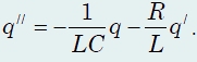

This equation is also familiar to us - this is the equation of damped oscillations

and the attenuation coefficient, as expected, is proportional to the active resistance of the circuit β = R/L.
The processes taking place in oscillatory circuit, can also be described using the law of conservation of energy. If we neglect the active resistance of the circuit, then the sum of the energies electric field capacitor and magnetic field coil remains constant, which is expressed by the equation

which is also an equation of harmonic oscillations with a frequency determined by formula (5). In its form, this equation also coincides with the equations following from the law of conservation of energy during mechanical vibrations. Since the equations describing the oscillations electric charge capacitor are similar to the equations describing mechanical vibrations, then we can draw an analogy between the processes occurring in the oscillatory circuit and the processes in any mechanical system. On fig. 672 such an analogy has been drawn for oscillations mathematical pendulum. In this case, the analogs are "capacitor charge q(t)− pendulum deflection angle φ(t)” and “current I(t) = q / (t)− pendulum speed V(t)».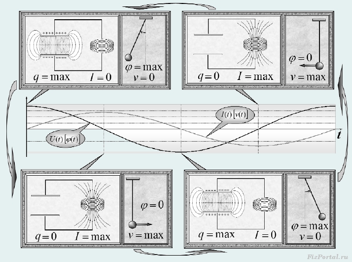



rice. 672
Using this analogy, we qualitatively describe the process of charge oscillations and electric current in contour. At the initial moment of time, the capacitor is charged, the strength of the electric current is zero, all the energy is contained in the energy of the electric field of the capacitor (which is similar to the maximum deviation of the pendulum from the equilibrium position). Then the capacitor begins to discharge, the current strength increases, while the self-induction EMF occurs in the coil, which prevents the current from increasing; the energy of the capacitor decreases, turning into the energy of the magnetic field of the coil (an analogy - the pendulum moves towards bottom point with increasing speed). When the charge on the capacitor becomes zero, the current strength reaches its maximum value, while all the energy is converted into the energy of the magnetic field (the pendulum has reached its lowest point, its speed is maximum). Then the magnetic field begins to decrease, while the self-induction EMF maintains the current in the same direction, while the capacitor begins to charge, and the signs of the charges on the capacitor plates are opposite to the initial distribution (analogue - the pendulum moves to the opposite initial maximum deviation). Then the current in the circuit stops, while the charge of the capacitor again becomes maximum, but opposite in sign (the pendulum has reached its maximum deviation), after which the process will be repeated in the opposite direction.

LECTURE #8

Mechanics

fluctuations

oscillatory movement. Kinematic and dynamic characteristics of oscillatory motion. Mathematical, physical and spring pendulum.

We live in a world where oscillatory processes are an integral part of our world and are found everywhere.

An oscillatory process or oscillation is a process that differs in one degree or another of repetition.

If an oscillating value repeats its values ​​at regular intervals, then such oscillations are called periodic, and these periods of time are called the oscillation period.

Depending on the physical nature of the phenomenon, oscillations are distinguished: mechanical, electromechanical, electromagnetic, etc.

Fluctuations are widespread in nature and technology. Oscillatory processes underlie some branches of mechanics. In this course of lectures, we will only talk about mechanical vibrations.

Depending on the nature of the impact on the oscillatory system, oscillations are distinguished: 1. Free or natural, 2. Forced oscillations, 3. Self-oscillations, 4. Parametric oscillations.

Free oscillations are called oscillations that occur without external influence and are caused by the initial “push”.

Forced vibrations occur under the action of a periodic external force

Self-oscillations are also performed under the action of an external force, but the moment of the force's action on the system is determined by the oscillatory system itself.

With parametric oscillations due to external influences, a periodic change in the parameters of the system occurs, which causes this type of oscillation.

The simplest form is harmonic vibrations

Harmonic vibrations are vibrations that occur according to the lawsin orcos . An example of harmonic oscillations is the oscillation of a mathematical pendulum

The maximum deviation of an oscillating quantity in the process of oscillation is called oscillation amplitude(BUT) . The time it takes to complete one complete oscillation is called period of oscillation(T) . The reciprocal of the period of oscillation is called oscillation frequency(). Often fluctuations multiplied by 2 is called cyclic frequency(). Thus, harmonic oscillations are described by the expression

Here ( t+  0 ) oscillation phase, and  0 - initial phase

The simplest mechanical oscillatory systems are the so-called: mathematical, spring and physical pendulums. Let's take a closer look at these pendulums.

8.1. Mathematical pendulum

A mathematical pendulum is an oscillatory system consisting of a massive point body suspended in the field of gravity on an inextensible weightless thread.

At the bottom point, the pendulum has a minimum of potential energy. Let's deflect the pendulum at an angle  . The center of gravity of a massive point body will rise to a height  h and in this case the potential energy of the pendulum will increase by the value mg h. In addition, in the deflected position, the weight is affected by gravity and the tension of the thread. The lines of action of these forces do not coincide, and the resultant force acts on the load, tending to return it to the equilibrium position. If the load is not held, then under the action of this force it will begin to move to the initial equilibrium position, its kinetic energy will increase due to an increase in speed, while the potential energy will decrease. When the equilibrium point is reached, the resultant force will no longer act on the body (the force of gravity at this point is compensated by the force of the thread tension). The potential energy of the body at this point will be minimal, and the kinetic energy, on the contrary, will have its own maximum value. The body, moving by inertia, will pass the equilibrium position and begin to move away from it, which will lead to the emergence of a resultant force (from tension and gravity), which will be directed against the movement of the body, slowing it down. This starts a decrease kinetic energy cargo and its increase potential energy. This process will continue until the complete exhaustion of the kinetic energy reserves and its transition to potential energy. In this case, the deviation of the load from the equilibrium position will reach a maximum value and the process will be repeated. If there is no friction in the system, the load will oscillate indefinitely.

Thus, oscillatory mechanical systems are characterized by the fact that when they deviate from the equilibrium position, a restoring force arises in the system, which tends to return the system to the equilibrium position. In this case, oscillations occur accompanied by a periodic transition of the potential energy of the system into its kinetic energy and vice versa.

Calculate oscillatory process. Moment of forces M acting on the pendulum is obviously equal to - mglsin The minus sign reflects the fact that the moment of forces tends to return the load to its equilibrium position. On the other hand, according to the basic law rotary motion M=ID 2  / dt 2 . Thus, we get the equality

B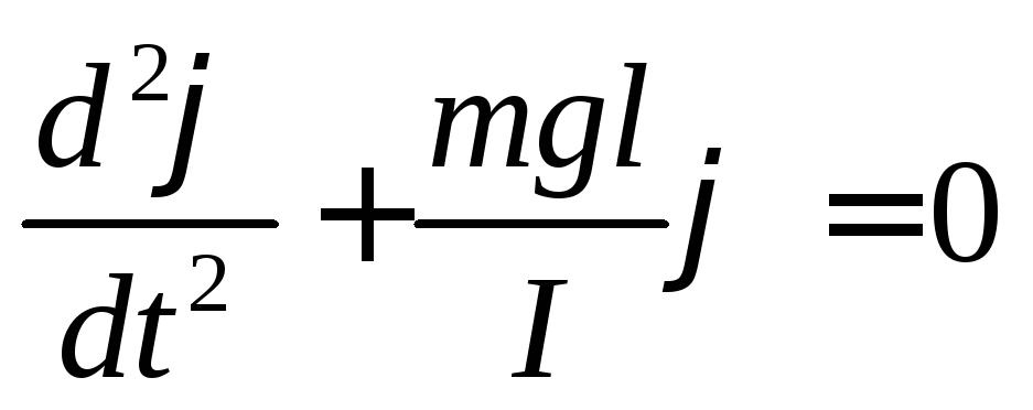

Let us consider only small angles of deviation of the pendulum from the equilibrium position. Then sin ≈  . And our equality will take the form:

D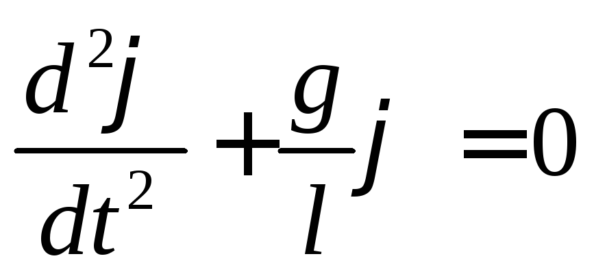

for a mathematical pendulum it is true I= ml 2 . Substituting this equality into the resulting expression, we obtain an equation describing the process of oscillation of a mathematical pendulum:

This differential equation describes an oscillatory process. The solution to this equation is the harmonic functions sin( t+  0 ) or cos ( t+  0 ) Indeed, we substitute any of these functions into the equation and get:  2 = g/ l. Thus, if this condition is met, then the functions sin( t+  0 ) or cos( t+  0 ) turn the differential equation of oscillations into an identity.

O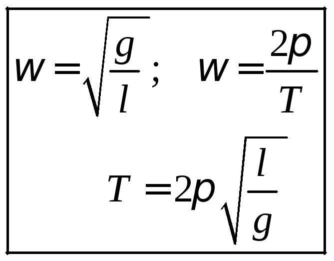

here the cyclic frequency and period of oscillation of a harmonic pendulum is expressed as:

The oscillation amplitude is found from the initial conditions of the problem.

As you can see, the frequency and period of oscillation of a mathematical pendulum do not depend on the mass of the load and depend only on the acceleration of gravity and the length of the suspension thread, which allows the pendulum to be used as a simple but very accurate device for determining the acceleration of gravity.

Another type of pendulum is any physical body suspended from any point of the body and having the ability to perform oscillatory motion.

8.2. physical pendulum

AT Let's take an arbitrary body, pierce it at some point with an axis that does not coincide with its center of mass, around which the body can freely rotate. Suspend the body on this axis, and deviate it from the equilibrium position by some angle  .

T

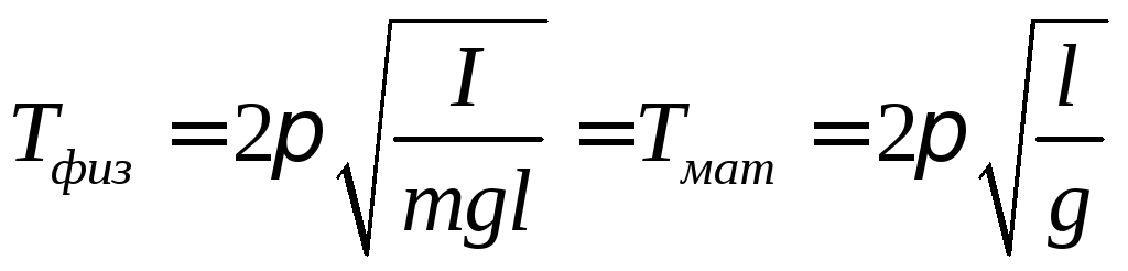
when on a body with a moment of inertia I about the axis O the moment returning to the equilibrium position will act M = - mglsin and the oscillations of a physical pendulum, as well as a mathematical one, will be described by a differential equation:

Since for different physical pendulums the moment of inertia will be expressed differently, we will not describe it as in the case of a mathematical pendulum. This equation also has the form of an oscillation equation, the solution of which are functions describing harmonic oscillations. In this case, the cyclic frequency ( ) , oscillation period (T) defined as:

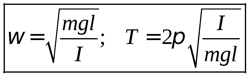
We see that in the case of a physical pendulum, the oscillation period depends on the geometry of the pendulum body, and not on its mass, as in the case of a mathematical pendulum. Indeed, the expression for the moment of inertia includes the mass of the pendulum to the first power. The moment of inertia in the expression for the oscillation period is in the numerator, while the mass of the pendulum is included in the denominator and also in the first degree. So the mass in the numerator cancels out with the mass in the denominator.

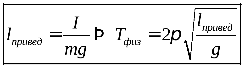
The physical pendulum has one more characteristic - the reduced length.

The reduced length of the physical pendulum is the length of the mathematical pendulum, the period of which coincides with the period of the physical pendulum.

This definition makes it easy to define an expression for the reduced length.

Comparing these expressions, we get

If on the line drawn from the point of suspension through the center of mass of the physical pendulum we plot (starting from the point of suspension) the reduced length of the physical pendulum, then at the end of this segment there will be a point that has a remarkable property. If a physical pendulum is suspended from this point, then its oscillation period will be the same as in the case of suspension of the pendulum at the previous suspension point. These points are called the swing centers of the physical pendulum.

Consider another simple oscillatory system that performs harmonic oscillations

8.3. Spring pendulum

P 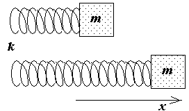imagine that by the end of the spring with the stiffness coefficient k weight attached m.

If we move the load along the x axis by stretching the spring, then the force returning to the equilibrium position will act on the load F return = - kx. If the load is released, then this force will cause acceleration d 2 x / dt 2 . According to Newton's second law, we get:

md 2 x / dt 2 = - kx from this equation we obtain the equation for the oscillation of a load on a spring in its final form: d 2 x / dt 2 + (k/ m) x = 0

E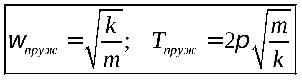

then the oscillation equation has the same form as the oscillation equations in the cases already considered, which means that the solution to this equation will be the same harmonic functions. The frequency and period of oscillations will be respectively equal

Moreover, the force of gravity in no way affects the oscillations of the spring pendulum. Since in this case it is a constantly acting factor, acting all the time in one direction and having nothing to do with the restoring force.

Thus, as we see the oscillatory process in a mechanical oscillatory system, it is characterized primarily by the presence in the system restoring force acting on the system, and the oscillations themselves are characterized by: amplitude of fluctuation by their period, frequency and phase of fluctuations.