n1.doc
The main types of local resistance.Determination of the local loss factor
Chapter 3 has already considered the issue of calculating pressure losses at local resistances, that is, such sections of the pipeline where, due to a change in the size or configuration of the channel, the flow velocity changes, it separates from the walls and vortices appear. Consider local resistance in more detail.
The simplest local hydraulic resistances can be divided into three groups: expansions, narrowings, and channel turns. Each of them can be sudden or gradual. More difficult cases local resistances are combinations of these simplest resistances. For example, in a valve, the flow first curves, narrows, and finally expands.
At turbulent mode flow, the loss coefficients are determined mainly by the form of local resistances, and practically do not depend on the Reynolds number Re, therefore, the magnitude of local losses is proportional to the square of the velocity. This relationship is called quadratic. The values of the loss coefficients are found mainly empirically, although for some of the simplest local resistances they can be obtained theoretically. When deciding practical tasks values are found in reference books, where they are given in the form of formulas, tables, graphs for various kinds local resistance.
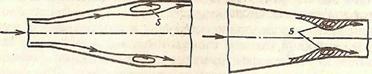
For most local resistances in pipelines at Re 10 5, turbulent self-similarity takes place - the head loss is proportional to the velocity to the second power and the local resistance coefficient does not depend on Re. In local resistance where going abrupt change section of the pipeline and significant vortices are formed, self-similarity is established even at Re 10 4 . For example, for a sudden expansion of a pipeline, where S 1 and S 2 – pipeline areas before and after sudden expansion. To exit the pipeline to the tank S 2 >> S 1 , therefore m 1. With a gradual expansion of the flow in the diffuser, the coefficient of local resistance
 ,
,
where d is the loss factor.
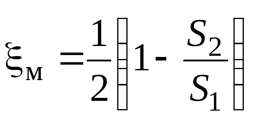
With a sudden narrowing of the pipe  . To enter the pipeline from the tank S 1 >> S 2 , so m 0.5.
In a laminar flow regime, local losses are usually small compared to friction losses, and the drag law is more complex than in a turbulent regime:
where h tr - head loss caused directly by the action of friction forces (viscosity) in a given local resistance and proportional to the viscosity of the fluid and velocity to the first degree; h vortex - losses associated with flow separation and vortex formation in the local resistance itself or behind it and proportional to the speed to the second degree.
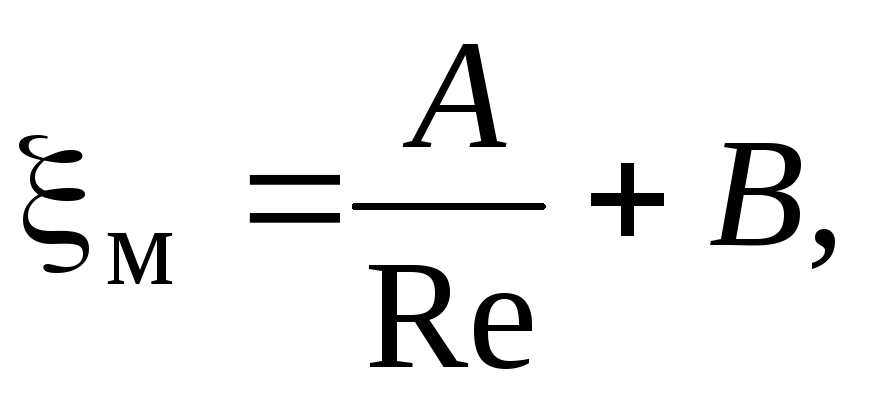
Thus, the loss factor in laminar flow can be represented as the sum of:
where A and B are dimensionless constants that depend mainly on the form of local resistance.
Depending on the value of Re and the shape of the local resistance, the head loss in laminar mode can be expressed as a linear or quadratic dependence on the speed, as well as some average curve between them. Coefficient values A and B should be searched in the reference book depending on the type of local resistance and its parameters.
Local losses and coefficient of local resistance.
Pipeline networks that distribute or discharge liquid from consumers change their diameter (section); turns, branches are arranged on the networks, locking devices are installed, etc. In these places, the flow changes its shape and sharply deforms. Due to the change in shape, additional resistance forces arise, so called local resistance. It takes effort to overcome them. The pressure expended to overcome local resistances is called local pressure losses and denoted by  .
.
The local head loss is defined as the product of the velocity head immediately adjacent to the local resistance  ,
according to the formula
,
according to the formula
There is no general theory for determining the coefficients of local resistance, with the exception of individual cases. Therefore, the coefficients of local resistance, as a rule, are found empirically. Their meanings for various elements pipelines are given in technical handbooks. Sometimes local resistances are expressed in terms of the equivalent length of a straight pipeline section.  . Equivalent length called such a length of a straight section of a pipeline of a given diameter, the pressure loss in which, when a given flow is passed, is equal to the considered local losses. Equating the Darcy-Weisbach formulas and (1), we have , we get , or .
The main characteristics of the outflow of liquid through holes and nozzles (Toricelli's formula; types of outflow; coefficients of compression, velocity and flow; types of jet compression).
Classification of holes and their practical application
The issue of fluid flow through holes is one of the key moments of hydraulics. Scientists and engineers have been studying this issue since 17th century D. Bernoulli's equation was first derived when solving one of the problems on the outflow of fluid from a hole. When calculating diaphragms, perforated mixers, filling and emptying tanks, pools, reservoirs, lock chambers and other containers, problems are solved for the outflow of liquids through holes. When solving these problems, the speeds and flow rates of liquids are determined.
It has been experimentally established that when the liquid flows out of the holes, the jet is compressed, i.e., its decrease cross section. The shape of the compressed jet depends on the shape and size of the hole, the thickness of the walls, and also on the location of the hole relative to the free surface, walls and bottom of the vessel from which the liquid flows. The compression of the jet occurs due to the fact that the liquid particles approach the hole with different sides and move by inertia in the hole along converging trajectories.
The parallel flow of jets in the hole is possible only when the thickness of the walls of the vessel is close to the size of the hole, and the walls of the hole have smooth outlines, with expansion into the vessel. In this case, the hole turns into a conoidal deposit (see below).
Holes are classified as follows:
1. By size.
BUT 
) small holes when  or
or  (Fig. 38), where
  is the diameter of the round hole;
  - pressure;
  - pressure difference with a flooded hole;
b) big holes  or
or  .
.
2. According to the thickness of the wall in which the hole is made:
A) holes in a thin wall, when  or
or  ,
where t –
wall thickness;
,
where t –
wall thickness;
B) holes in a thick wall, when  or
or  .
.
3. The shape distinguish between round, square, rectangular, triangular and other holes
Types of nozzles and their application. Fluid flow through nozzles
nozzle A piece of pipe is called, the length of which is several times the inner diameter. Let us consider the case when a nozzle with a diameter of d,
equal to the hole diameter.
On fig. 44 shows the most common types of nozzles used in practice:
a - cylindrical outer; b- cylindrical internal; in - conical divergent; G- conical converging; d - conoidally divergent; e - conoidal.
C 
cylindrical nozzles are found in the form of parts hydraulic systems machines and structures. Conical converging and conoidal nozzles are used to increase the speed and range of a water jet (fire hoses, hydraulic monitor barrels, nozzles, nozzles, etc.).
To  conical diverging nozzles are used to reduce the speed and increase the fluid flow and outlet pressure in the suction pipes of turbines, etc. Ejectors and injectors also have conical nozzles as the main working body. Culverts under road embankments (in terms of hydraulics) are also nozzles.
Let us consider the outflow through an external cylindrical nozzle (Fig. 45).
The jet of liquid at the entrance to the nozzle is compressed, and then expands and fills the entire section. The jet flows out of the nozzle with a full cross section, so the compression ratio, referred to the outlet cross section,  , and the flow rate
 .
.
We compose the D. Bernoulli equation for the sections 1-1 and 2-2
 ,
,
Where  - pressure loss.
For an outflow from an open reservoir into the atmosphere, similarly to an outflow through an orifice, the D. Bernoulli equation is reduced to the form
 . (144)
The pressure loss in the nozzle is the sum of the loss at the inlet and the expansion of the compressed jet inside the nozzle. (Insignificant losses in the reservoir and losses along the length of the nozzle, due to their smallness, can be neglected.) So,
 . (145)
According to the continuity equation, we can write:
 ,
,
Substituting value  into equation (145), we have
Where indicated
 . (148)
We substitute the obtained value of head loss into equation (144), then
 .
.
Hence the flow rate
 . (149)
denoting
 , (150)
We get the equation for the speed
 . (151)
Determine the fluid flow
 .
.
But for the nozzle  and
and
 , (152)
Where  – nozzle flow rate;
  - area of the active section of the nozzle.
Thus, the equations for determining the velocity and flow rate of liquid through the nozzles have the same form as for the orifice, but with different values of the coefficients. For the jet compression ratio (at large values R e
and  ) can be approximately taken
  , and then by formulas (148) and (149) we obtain
  . In fact, there are also losses along the length, therefore, for the outflow of water in normal conditions can be taken
  .
.
Comparing the flow and velocity coefficients for the nozzle and the hole in a thin wall, we find that the nozzle increases the flow rate and reduces the outflow rate.
A characteristic feature of the packing is that the pressure in the compressed section is less than atmospheric pressure. This position is proved by the Bernoulli equation, compiled for the compressed and outlet sections.
In the inner cylindrical nozzles, the jet compression at the inlet is greater than in the outer ones, and therefore the values of the flow rate and velocity coefficients are smaller. Experiments found coefficients for water  .
.
In external conical converging nozzles, the compression and expansion of the jet at the inlet is less than in external cylindrical ones, but external compression appears at the outlet of the nozzle. Therefore, the coefficients  and
and  depend on the taper angle. With an increase in the taper angle to 13°, the flow coefficient increases, and with a further increase in the angle it decreases.
Converging converging nozzles are used in cases where it is necessary to obtain a high output jet speed, flight range and jet impact force (hydraulic monitors, fire nozzles, etc.).
In conical diverging nozzles internal extension jets after compression are larger than in conical converging and cylindrical ones, so the head loss here increases and the velocity coefficient decreases. There is no external compression on exit.
The coefficients and depend on the taper angle. So, at the taper angle  the values of the coefficients can be taken equal to
  ; at
; at  (limit angle)
  . At
. At  the jet flows out without touching the walls of the nozzle, i.e., as from a hole without a nozzle.
Liquid leakage from holes and nozzles
7.1. Flow through a small hole in a thin wall
with constant pressure
Consider various occasions liquid outflows from reservoirs, tanks, boilers, etc. through holes and nozzles into the atmosphere or into a space filled with a gas or the same liquid. With such an expiration potential energy liquids in larger or lesser degree turns into kinetic energy jets. We are mainly interested in two outflow parameters: velocity and flow rate.
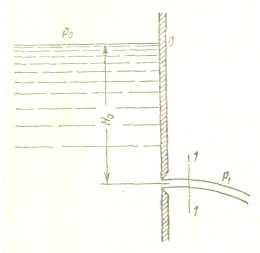
Let the liquid be in a large pressurized tank p 0 (Fig. 29). In its wall at a sufficiently large depth from the free surface H 0 there is a small round hole through which the liquid flows into the air (gas) space with pressure p 1 .
Let the hole have the shape shown in Fig. 30, that is, this drilling in a thin wall without processing the leading edge or is made in a thick wall, but the leading edge is sharpened with outside.
Rice. 29. Expiration from
reservoir through a small
hole 
Rice. 30. Outflow through the round
hole
Liquid particles approach the hole from the entire adjacent volume, moving rapidly along various smooth trajectories. The jet breaks away from the wall at the edge of the hole and then contracts somewhat. The jet acquires a cylindrical shape approximately at a distance of one hole diameter from the inlet edge. The reason for the compression of the jet is the inertia of the liquid. Since the hole size is small compared to the head H 0 and the dimensions of the reservoir, and therefore, its side walls and free surface do not affect the flow of liquid to the hole, then perfect compression jets, that is, the largest.
The compression ratio is estimated by the jet compression ratio
Let us write down the Bernoulli equation for the free surface (section 0 – 0) and the section of the jet, where it has assumed a cylindrical shape (section 1 – 1):
The fluid velocity in the 0 – 0 section can be neglected. Let's introduce the calculated head

where is the speed coefficient:
If the liquid is ideal, then = 0, and = 1, therefore, = 1 and the outflow velocity ideal fluid
Having considered the obtained expressions, it can be found that the velocity coefficient is the ratio of the actual outflow velocity to the velocity of an ideal fluid
The actual outflow velocity is always less than the ideal velocity due to drag, hence the velocity factor is always less than 1.
The distribution of velocities over the cross section of the jet is uniform only in its middle part, and outer layer liquid is somewhat slowed down due to friction against the wall. Experiments show that in the core of the jet the exhaust velocity is almost equal to the ideal V and, therefore, the introduced speed coefficient should be considered as a coefficient average speed.
Let's calculate the volume flow
The product = is the flow coefficient. Then finally
where p- the calculated pressure difference, under the action of which the outflow occurs.
The complexity of using this expression lies in the exact estimation of the flow coefficient . It's clear that

This means that the flow rate is the ratio of the actual flow rate to the flow rate that would occur in the absence of jet compression and resistance. is not the flow rate of an ideal fluid, since compression of the jet will also be observed for an ideal fluid.
The actual flow rate is always less than the theoretical flow rate and hence the flow rate factor is always less than 1 due to jet compression and drag. Sometimes one factor is more important, sometimes another.
The coefficients , , and depend, first of all, on the type of hole or nozzle, and also, like all dimensionless coefficients in hydraulics, on the main criterion of hydrodynamic similarity - the Re number.
The nature of the change in the coefficients , and for a round hole from Re and calculated from the ideal outflow velocity
 ,
,
shown in Fig. 31.
It can be seen from the graph that with an increase in Re and, that is, with a decrease in the influence of viscous forces, the coefficient increases due to a decrease in the drag coefficient , and the coefficient decreases due to a decrease in fluid deceleration at the edge of the hole and an increase in the radii of curvature of the jet surface in its section from edges to the beginning of the cylindrical section. The values of the coefficients and in this case asymptotically approach the values corresponding to the outflow of an ideal fluid, that is, for Re and the values 1, and 0.6. The flow coefficient with an increase in Re and first increases, due to a steep increase in , and then, having reached a maximum ( max = 0.69 at Re and = 350), decreases due to a significant drop in and at large values of Re and practically stabilizes at the value = 0.60 0.61. 
Rice. 31. Dependence of , and on Re and for a round hole
in a thin wall
In the region of very small values of Re and (Re and 
For low-viscosity liquids (water, gasoline, kerosene, etc.), the outflow of which usually occurs when large numbers Re, the outflow coefficients vary within narrow limits. Usually, the following averaged values are taken into account: ( = 0.64; = 0.97; = 0.62; = 0.065).
7.2. Outflow through nozzles
External cylindrical nozzle(Fig. 32) is called a short tube with a length equal to several diameters without rounding the leading edge. In practice, such nozzles are often obtained in cases where drilling is performed in a thick wall and the leading edge is not processed.
The outflow through such nozzles in gaseous environment can happen in two ways. The first expiration mode is shown in the first and second figures, and the second in the third. In the first mode, the jet after entering the nozzle is compressed approximately in the same way as when it flows through the nozzle in a thin wall. Then, due to the interaction of the compressed part of the jet with the surrounding
Rice. 32. Outflow through the outer cylindrical nozzle
swirling liquid, the jet gradually expands to the size of the hole and leaves the nozzle with a full cross section. This mode of expiration is called continuous.
Since at the outlet of the nozzle the jet diameter is equal to the diameter of the hole, then = 1 and, consequently, = . The averaged values of the coefficients for this regime of outflow of low-viscosity liquids (for large Re) are as follows:
= = 0.8; = 0.5.
In this flow mode, compared to the flow from a hole in a thin wall, the flow rate is higher due to the lack of jet compression at the nozzle exit, and the velocity is lower due to the greater resistance. The following empirical formula can be recommended to calculate the flow rate for continuous flow:
It follows from the formula that when Re = max = 0.813.
Minimum relative nozzle length l/d, at which the first expiration mode can be realized, is approximately equal to 1. However, even for sufficient values l/d this mode is not always possible.
Let us find the pressure inside the nozzle and the condition under which a continuous flow regime is possible.
Let the outflow occur under the action of pressure p 0 in a gas environment with pressure p 2. The calculated pressure in this case is equal to
Since the pressure at the outlet of the nozzle p 2 , in the narrowed section 1–1, where the velocity is higher, the pressure p 1 p 2 . However, the more pressure H, and hence the cost Q, the lower the pressure p 2. Pressure difference p 2 – p 1 grows in proportion to the pressure H. Let's write the Bernoulli equation and see this:

where the last term of the equation is the pressure loss on the expansion of the flow, which in this case occurs in much the same way as with a sudden expansion of the pipeline.
Speed ratio
Eliminate from the Bernoulli equation V 1 using this relation and replace ![]() and find the pressure drop inside the nozzle:
and find the pressure drop inside the nozzle:
Substituting = 0.8 and = 0.63, we get p 2 – p 1 0.75 g H.
At some critical pressure H cr absolute pressure inside the nozzle becomes equal to the pressure saturated vapors, that's why

if we neglect the saturation vapor pressure. Therefore, at H > H kr pressure p 1 must become negative, which cannot be, so the non-separated expiration mode at H > H kr becomes impossible and there is a transition to the second expiration mode.
The second mode of flow is characterized by the fact that the jet, after compression, no longer expands, but retains its cylindrical shape and moves inside the nozzle without touching its walls. The outflow becomes exactly the same as from a hole in a thin wall. Consequently, in the transition from the non-separated flow regime to the separated one, there is an increase in the velocity and a decrease in the flow rate. If water flows out into the atmosphere through an external cylindrical nozzle, then

If the pressure is reduced in the second expiration mode, then this mode will remain until the smallest H. This means that the second flow mode is possible at any pressure, and at H H cr both modes of expiration are possible.
When flowing through a cylindrical nozzle under the level, the first mode will not differ from that described above, but when the absolute pressure increases H drops to the saturated vapor pressure, there will be no transition to the second mode, and the cavitation mode sets in, at which the flow rate ceases to depend on the backpressure p 2, that is, the stabilization effect appears. In this case, the lower the relative backpressure
 ,
,
the wider the cavitation area inside the nozzle and the less ratio consumption .
Thus, the external cylindrical nozzle has significant disadvantages: in the first mode - great resistance and an insufficiently high flow coefficient, and on the second, a very low flow coefficient. In addition, the duality of the regime of outflow into a gaseous medium at H H cr, ambiguity of flow rate at a given H and the possibility of cavitation when flowing below the level.
The outer cylindrical nozzle can be greatly improved by rounding the entry lip or arranging a conical entry with a taper angle of about 60. How more radius rounding, the lower the drag coefficient and the higher the flow coefficient. In the limit, with a radius equal to the wall thickness, such a nozzle approaches the conoidal nozzle, or nozzle.
Rice. 33. Conoidal nozzle (nozzle)
Conoid nozzle (nozzle) shown in Fig. 33, is outlined approximately in the form of a naturally compressible jet and due to this ensures the continuity of the flow inside the nozzle and the parallel jet in its outlet section. This is a widely used packing, as it has a flow coefficient close to 1 and very low losses, as well as a stable flow regime without cavitation. For him = 0.03 0.1; = = 0.96 0.99.
Rice. 34. Diffuser nozzle
Diffuser nozzle
Local resistances include short sections of pipes in which there is a change in the speed of fluid movement in magnitude and direction. The simplest local resistances can be conventionally divided into resistances caused by a change in the flow cross section (expansion, narrowing), and resistances associated with a change in the direction of fluid movement. But most of the local resistances are combinations of these cases, since the rotation of the flow can lead to a change in its cross section, and the expansion (narrowing) of the flow can lead to a deviation from the rectilinear motion of the fluid. Also, various hydraulic fittings (faucets, valves, valves, etc.) are practically always a combination of the simplest local resistances. Local resistances also include sections of pipelines with separation or merging of fluid flows. Local resistances have a significant impact on the operation of hydraulic systems with turbulent fluid flows. With laminar flows, in most cases these head losses are small compared to the frictional losses in pipes. In most local resistances, a change in the speed of movement leads to the emergence of vortices, which use the energy of the fluid flow for their rotation. Thus, vortex formation is the main cause of head loss in most local resistances. Weisbach's formula is used to determine these losses: For a sudden expansion of the flow, S1 is the cross-sectional area of the flow before the expansion, S2 is after the expansion. - dimensionless coefficient of local resistance.
If liquid flows out of the pipe into the tank, then
1 because S1 For a sudden narrowing of the flow: . If the liquid flows out of the tank through the pipe (S1>S2), then . With a gradual narrowing and expansion of the flow (the expanding channel is called a diffuser, narrowing - a confuser (if the confuser is a fused transition - a nozzle)). In addition to losses due to vortex formation, losses due to friction along the length are taken into account. and, where kp and kc are correction factors (values in reference books). There are also turns of streams: sudden and smooth. The sudden flow causes significant eddying. Their coefficients can be found in reference books. Holes in hydraulics are divided into small and large. Small holes, various points whose geometric head is the same. The shape of the holes in many cases significantly affects the parameters of the outflowing flow and its shape. The change in the shape of a flowing liquid jet relative to the hole is called fluid inversion. Holes can be made in thin or thick walls. The wall is considered thin, if its thickness is S<2/3
напора. thick wall, if S>2/3 head .
The phenomenon of jet compression through a hole in a thin wall at a certain distance: Jet compression ratio Compression is called perfect if the side walls of the vessel do not affect the outflow of the jet. Full - compression around the entire perimeter If H=const, then this is a confluence at a constant head Free flow of liquid - the outflow of liquid into the atmosphere. Velocity and fluid flow: , Speed for real liquid corrected using the coefficients , - speed coefficient. For flow: , - flow coefficient Local resistances are called, in contrast to resistances along the length, pressure losses concentrated on short sections of the pipeline, caused by local separation of vortices, as well as a violation of the flow structure. These processes largely depend on the form of local resistances. Conventionally, local resistances can be divided into several types, shown in Fig. 4.13 sudden expansion sudden contraction Diffuser Confuser Diaphragm Piping rounding Local resistances, in particular, include sections of pipelines that have transitions from one diameter to another, elbows, sockets, tees, crosses, all kinds of locking devices and devices (faucets, gate valves, valves, valves), as well as filters, grids, special inlet and outlet devices for pumps (diffusers, confusers). Accounting for local resistances plays a decisive role in the calculation of hydraulically short pipelines, where the amount of energy loss due to local resistances is comparable to the losses along the length. Virtually any local resistance leads to a sharp change in the nature of the current, accompanied by a change in local velocities, both in magnitude and in direction. In practice, to determine the energy loss at local resistances, it is used Weisbach formula, expressing losses in fractions of velocity head Where the unknown proportionality factor ζ is called coefficient of local resistance. as speed v the speed is taken on the pipeline section, or before it. This will depend numerical value coefficient ζ, therefore, it is necessary to specifically stipulate in relation to which speed the coefficient of local resistance is calculated. AT general case coefficient ζ depends on geometric shape local resistance and Re number. The coefficient ζ is assumed to be constant for a given type of local resistance. However, experimental studies have shown that this condition is met only at high Reynolds numbers (Re > 104), At small values of Re, the values of the coefficient ζ depend significantly on the Reynolds number, Reference values of ζ refer to the case when the local resistance operates under conditions of self-similarity in the Re number , i.e. does not depend on it numerical value. The values of ζ given in reference books should be considered indicative. To clarify the data on a specific local resistance, it is necessary to carry out pilot study in the required range of Re numbers. However, there are cases where the amount of energy loss due to local resistance can be theoretically determined, for example, with a sudden expansion of the flow. Sometimes local resistances are expressed in terms of the equivalent length of a straight pipeline section. . Equivalent length called such a length of a straight section of a pipeline of a given diameter, the pressure loss in which, when a given flow is passed, is equal to the considered local losses. Chapter 3 has already considered the issue of calculating pressure losses at local resistances, that is, such sections of the pipeline where, due to a change in the size or configuration of the channel, the flow velocity changes, it separates from the walls and vortices appear. Consider local resistance in more detail. The simplest local hydraulic resistances can be divided into three groups: expansions, narrowings, and channel turns. Each of them can be sudden or gradual. More complex cases of local resistances are combinations of these simplest resistances. For example, in a valve, the flow first curves, narrows, and finally expands. In a turbulent flow regime, the loss coefficients are determined mainly by the form of local resistances, and practically do not depend on the Reynolds number Re, therefore, the magnitude of local losses is proportional to the square of the velocity. This relationship is called quadratic. The values of the loss coefficients are found mainly empirically, although for some simple local resistances they can be obtained theoretically. When solving practical problems, the values of are found in reference books, where they are given in the form of formulas, tables, graphs for various types of local resistances. For most local resistances in pipelines at Re 10 5, turbulent self-similarity takes place - the head loss is proportional to the velocity to the second power and the local resistance coefficient does not depend on Re. In local resistances, where there is a sharp change in the cross section of the pipeline and significant vortices are formed, self-similarity is established even at Re 10 4 . For example, for a sudden expansion of a pipeline, where S 1 and S 2 – pipeline areas before and after sudden expansion. To exit the pipeline to the tank S 2
>> S 1 , therefore m 1. With a gradual expansion of the flow in the diffuser, the coefficient of local resistance where d is the loss factor. With a sudden narrowing of the pipe In a laminar flow regime, local losses are usually small compared to friction losses, and the drag law is more complex than in a turbulent regime: where h tr - head loss caused directly by the action of friction forces (viscosity) in a given local resistance and proportional to the viscosity of the fluid and velocity to the first degree; h vortex - losses associated with flow separation and vortex formation in the local resistance itself or behind it and proportional to the speed to the second degree. Thus, the loss factor in laminar flow can be represented as the sum of: where A and B are dimensionless constants that depend mainly on the form of local resistance. Depending on the value of Re and the shape of the local resistance, the head loss in laminar mode can be expressed as a linear or quadratic dependence on the speed, as well as some average curve between them. Coefficient values A and B should be searched in the reference book depending on the type of local resistance and its parameters. Local losses and coefficient of local resistance. Pipeline networks that distribute or discharge liquid from consumers change their diameter (section); turns, branches are arranged on the networks, locking devices are installed, etc. In these places, the flow changes its shape and sharply deforms. Due to the change in shape, additional resistance forces arise, so called local resistance. It takes effort to overcome them. The pressure expended to overcome local resistances is called local pressure losses and denoted by The local head loss is defined as the product of the velocity head immediately adjacent to the local resistance There is no general theory for determining the coefficients of local resistance, with the exception of individual cases. Therefore, the coefficients of local resistance, as a rule, are found empirically. Their values for various elements of pipelines are given in technical reference books. Sometimes local resistances are expressed in terms of the equivalent length of a straight pipeline section. The main characteristics of the outflow of liquid through holes and nozzles (Toricelli's formula; types of outflow; coefficients of compression, velocity and flow; types of jet compression).32. The outflow of liquid through a hole in a thin wall.

![]() , we get , or .
, we get , or .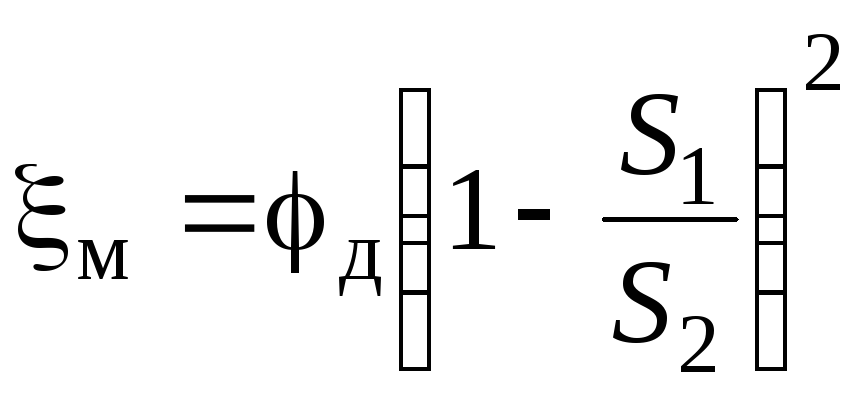 ,
, . To enter the pipeline from the tank S 1
>> S 2 , so m 0.5.
. To enter the pipeline from the tank S 1
>> S 2 , so m 0.5.
 .
. ,
according to the formula
,
according to the formula . (1)
. (1) .Equivalent length called such a length of a straight section of a pipeline of a given diameter, the pressure loss in which, when a given flow is passed, is equal to the considered local losses. Equating the Darcy-Weisbach formulas and (1), we have
 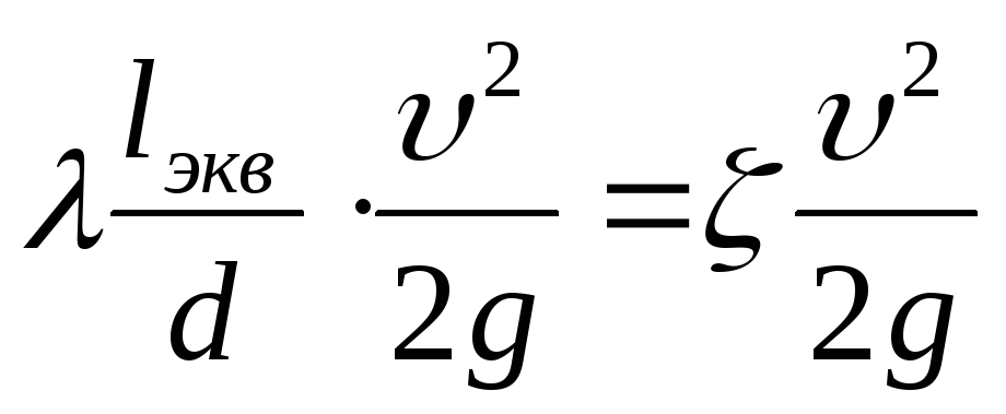 , we get
 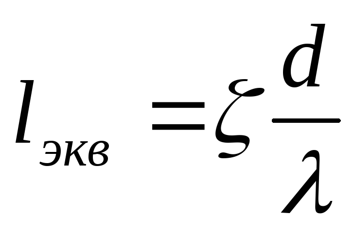 ,or
,or  .
.
